How ReaxFF Handles Bond Breaking and Formation: A Guide for Biomedical Researchers

Abstract

This article provides a comprehensive overview of the ReaxFF reactive force field, explaining its fundamental bond-order mechanism for simulating chemical reactions in complex molecular systems. Tailored for researchers and drug development professionals, it covers the methodology from foundational principles to practical application, parameterization, and troubleshooting. The content also explores validation protocols and compares ReaxFF's performance against quantum mechanical methods and emerging alternatives, highlighting its implications for simulating biochemical reactivity and drug design.

The Core Principle: Understanding ReaxFF's Bond-Order Concept

This technical guide provides a comprehensive examination of bond-order formalism and its quantum mechanical foundations, contextualized within reactive force field (ReaxFF) research. Bond order serves as a fundamental concept in chemistry, formally measuring the multiplicity of covalent bonds between atoms and providing critical insights into bond stability and strength. Originally introduced through Lewis's electron pair sharing concept and later quantified by Herzberg, Mulliken, and Hund as the difference between bonding and antibonding electron pairs, bond order has evolved into sophisticated computational definitions that accurately reflect diverse bonding environments. The development of ReaxFF represents a pivotal advancement in molecular simulation, employing bond-order formalism to enable dynamic modeling of bond breaking and formation processes at unprecedented scales. This review synthesizes current theoretical frameworks, computational methodologies, and practical applications of bond-order formalism, with particular emphasis on its implementation in ReaxFF and emerging approaches from quantum information theory and machine learning that are expanding the frontiers of reactive molecular dynamics research.

Foundations of Bond Order Theory

Historical Development and Fundamental Concepts

The concept of bond order originated from Gilbert N. Lewis's pioneering work on electron pairs shared between atoms, developed independently of quantum mechanics yet providing remarkable intuitive understanding of chemical bonding. This classical perspective was subsequently formalized by Herzberg, building on contributions from Mulliken and Hund, who defined bond order as "the difference between the numbers of electron pairs in bonding and antibonding molecular orbitals" [1]. In its most straightforward interpretation, bond order represents the number of electron pairs (covalent bonds) between two atoms, exemplified by the triple bond in N≡N (bond order = 3) or the double bond in O=O (bond order = 2) [1].

The earliest computational approaches to bond order assignment relied on heuristic electron assignment methods, including Lewis structures, valence shell electron pair repulsion (VSEPR) theory, and the concept of mesomerism for explaining aromaticity and multicenter bonding [2]. While these heuristic models continue to be valuable teaching tools due to their simple pictorial representations, they fundamentally lack universality because they assign bond orders in countable increments (whole numbers, half-numbers, etc.) while bond order properly exists on a continuous spectrum of non-negative real numbers [2]. This limitation necessitated the development of computational approaches that could capture the continuous nature of chemical bonding.

The Challenge of a Universal Definition

For decades, a satisfactory universal definition for bond order remained elusive despite the concept's widespread use throughout chemical sciences [2]. As noted by Manz, "a search for 'bond order' (with quotation marks) in Google Scholar returned 152,000 results," highlighting both the concept's popularity and the absence of consensus on its definition [2]. The fundamental challenge stems from the fact that as a material's geometry and electron cloud may be continuously deformed, the bond order must be allowed to vary continuously over the set of non-negative real numbers [2].

A significant advancement came with the recognition that for a material containing N electrons in the unit cell, a matrix BA,j can be defined where BA,j equals the number of electrons dressed-exchanged between an atom A in the reference unit cell and a particular atom j located anywhere in the material, with the constraint that the sum of all BA,j values equals N [2]. This framework provides a mathematical foundation for understanding bond order as a continuous variable while maintaining proper electron counting constraints.

Quantum Mechanical Origins of Chemical Bonding

The quantum origins of chemical bonding have been the subject of intensive theoretical investigation. Seminal work by Ruedenberg established that for H₂⁺ and H₂, roughly 66% of the binding energy could be associated with constructive quantum interference that lowers kinetic energy through electron delocalization across both centers [3]. This KE-lowering paradigm was long extrapolated to all covalent bonds, but recent research using variationally optimized absolutely localized molecular orbitals (ALMOs) has demonstrated that this generalization does not hold universally [3].

For bonds between heavier elements, such as H₃C–CH₃, F–F, H₃C–OH, H₃C–SiH₃, and F–SiF₃, kinetic energy often increases when radical fragments are brought together, contrary to the behavior observed in H₂⁺ and H₂ [3]. This difference originates from Pauli repulsion between the electrons forming the bond and core electrons, highlighting the fundamental role of constructive quantum interference (resonance) as the universal origin of chemical bonding, with differences between the interfering states distinguishing one type of bond from another [3].

Computational Methods for Bond Order Calculation

Numerous computational approaches have been developed to calculate bond orders from quantum chemical calculations, each with distinct theoretical foundations, advantages, and limitations. The following table summarizes key bond order methods referenced in current literature:

Table 1: Computational Methods for Bond Order Calculation

Method	Theoretical Basis	Key Features	Limitations
Mayer Bond Order (MBI) [4]	Function of first-order density matrix	Simple calculation; based on atom-atom overlap populations	Inconsistent across different quantum chemistry methods and SZ values of spin multiplet [2]
Wiberg Bond Index (WBI) [4]	Similar to MBI but in NAO basis	Stable with respect to basis set size; results align with formal valences	Primitive; relies on wavefunctions; limited to linear molecules for σ/π/δ decomposition
Laplacian Bond Order (LBO) [4]	Weighted integral of Laplacian of electron density	Matches chemical intuition; correlates with bond dissociation energy	Basis set dependent; only captures covalent interactions; currently limited to two-body interactions
DDEC6 Bond Order [2] [5]	Electrons dressed-exchanged between atoms	Works for diverse materials (molecular/periodic, localized/delocalized electrons); consistent across quantum methods	Does not apply to electrides, highly time-dependent states, some high-energy excited states [2]
Orbital Occupancy-Perturbed Mayer Bond Order [4]	Modification of MBI	Addresses some limitations of standard MBI	Limited testing across diverse systems
Fuzzy Bond Order [4]	Fuzzy partitioning of space	Alternative approach to bond order calculation	Less established compared to other methods
Intrinsic Bond Strength Index [4]	Energy decomposition analysis	Focuses on bond strength rather than electron counting	Different conceptual basis from electron-based bond orders

The DDEC6 Approach: A Comprehensive Method

A significant advancement in bond order computation came with the introduction of the DDEC6 method, which provides a comprehensive approach to computing bond orders from quantum mechanically computed electron and spin magnetization density distributions [2]. This method defines the bond order BA,B between atoms A and B in a material as the quantity of electrons dressed-exchanged between them, expanded as:

BA,B = CEA,B + ΛA,B

where CEA,B is the contact exchange and ΛA,B quantifies bond-order contributions arising from exchange hole delocalization [5]. The method is computationally efficient, derives from first principles, applies to numerous bonding types and diverse materials, and yields consistently accurate results across different quantum chemistry methods and different SZ values of a spin multiplet [5].

The DDEC6 approach successfully addresses key challenges in bond order computation, including handling non-magnetic, collinear magnetic, and non-collinear magnetic materials with localized or delocalized bonding electrons, working with non-equilibrium structures (stretched/compressed bonds, transition states), and functioning with any basis set type while maintaining low basis set sensitivity [2] [5]. This comprehensive capability represents a significant advancement over prior approaches, which struggled with one or more of these challenges.

Bond Order Trends in Diatomic Molecules

Systematic studies of bond orders across diatomic molecules have revealed important periodic trends and validated computational methods. Research on 288 diatomic molecules and ions has demonstrated that bond orders correlate with bond energies for elements within the same chemical group, while semicore electrons weaken bond orders for elements having diffuse semicore electrons [5]. These studies have also resolved long-standing debates about specific molecules, such as C₂, showing through DDEC6 analysis that its bond order is approximately 2.65, intermediate between the double bond in ethylene and triple bond in acetylene [5].

Table 2: Selected Diatomic Molecule Bond Orders Calculated with DDEC6 Method

Molecule	Spin Multiplicity	Bond Order	Notes
H₂	1	0.938	Near-unity bond order as expected
C₂	1	~2.65	Resolves long-standing debate
N₂	1	~3.0	Ideal triple bond confirmed
O₂	3	~2.0	Double bond with triplet spin state
F₂	1	~1.0	Single bond as expected
Mo₂	1	4.12	Quadruple bond characteristics

Quantum Information Theory Approaches

Recent work has explored chemical bonding through the lens of quantum information theory, introducing maximally entangled atomic orbitals (MEAOs) whose entanglement pattern recovers both Lewis (two-center) and beyond-Lewis (multicenter) structures [6]. In this framework, multipartite entanglement serves as a comprehensive index of bond strength, providing a unifying perspective for bonding analyses that is effective for equilibrium geometries, transition states in chemical reactions, and complex phenomena such as aromaticity [6].

This approach leverages parallels between chemical bonding and quantum entanglement, offering a QIT-based framework that captures crucial features of chemical bonding such as hybridization, bond orders, multicenter bonding, conjugation, and aromaticity without a priori chemical assumptions [6]. The method shows particular promise for addressing ambiguities in molecular orbital-based approaches, especially in multicenter molecules where traditional categorization of orbitals as bonding, antibonding, or nonbonding becomes arbitrary and potentially erroneous [6].

Bond-Order Formalism in ReaxFF

Theoretical Foundation of ReaxFF

The Reactive Force Field (ReaxFF) represents a pivotal application of bond-order formalism in molecular dynamics simulations. ReaxFF is a bond order (BO)-dependent force field whose core strength lies in its ability to dynamically handle bond breaking and formation during simulations, providing natural reaction trajectories [7]. Within the ReaxFF framework, all bonding-related energy terms are expressed as functions of the instantaneous bond order, ensuring energies smoothly approach zero upon bond dissociation [7].

The total system energy (Esystem) in ReaxFF comprises contributions from bond energy (Ebond), over-coordination energy (Eover), under-coordination energy (Eunder), valence angle energy (Eval), torsion angle energy (Etors), and non-bonded interactions (vdWaals and Coulomb) [7]. Critically, all bonding terms depend on bond orders, which are continuously updated during simulations based on interatomic distances, enabling the description of bond dissociation and formation.

Implementation of Bond-Order Formalism in ReaxFF

In ReaxFF, bond orders between atom pairs are calculated based on interatomic distances, typically using a empirical relationship that decreases smoothly as distance increases. This continuous bond-order formulation allows ReaxFF to naturally describe bond breaking and formation without additional switching functions or predefined reaction pathways. The bond-order dependence extends to angle and torsion terms, ensuring proper energy conservation as molecular connectivity changes during reactions.

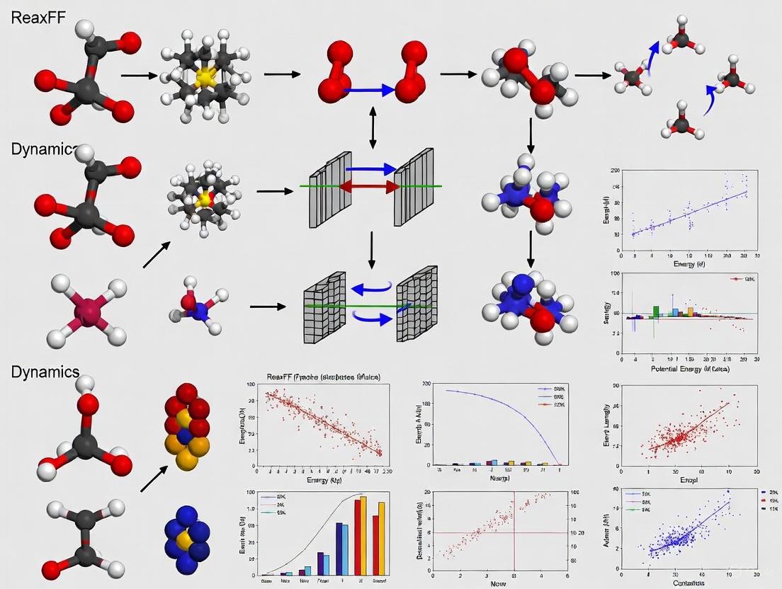
The following diagram illustrates how ReaxFF utilizes bond order formalism to simulate reactive processes:

Recent Advances in ReaxFF Parameterization

Recent research has expanded ReaxFF parameterization to increasingly complex systems. For instance, the development of a ReaxFF potential for lanthanum-carbon systems (ReaxFFCLa) has enabled investigation of lanthanum-based endohedral metallofullerenes (La-EMFs) formation mechanisms [7]. This parameterization retained the original ReaxFFC-2013 force field for carbon systems while developing new parameters for lanthanum, with validation against multiple quantum chemical benchmark systems showing excellent agreement with DFT calculations in terms of energy and geometry [7].

Molecular dynamics simulations using this force field revealed optimal conditions for La-EMF formation (C:La ratio of 12.5:1 and temperature of 2600 K) and identified that helium gas promotes cage formation while suppressing cage expansion [7]. Such studies demonstrate how bond-order formalism in ReaxFF enables investigation of complex reaction mechanisms that are challenging to study experimentally due to difficulties in real-time tracking of formation at nanosecond timescales and atomic resolution [7].

Comparative Analysis: Bond-Order Formalisms vs. Alternative Approaches

Performance Across Bonding Types

A critical assessment of bond order methods reveals significant variation in their performance across different bonding types. The DDEC6 approach has demonstrated accuracy across metallic, covalent, polar-covalent, ionic, aromatic, dative, hypercoordinate, electron deficient multi-centered, agostic, and hydrogen bonding [2]. This breadth of applicability surpasses earlier methods, which often exhibited severe limitations for specific bonding types.

For example, the occupancy bond index (OBI), defined as (sum of bonding orbital occupancies - sum of anti-bonding orbital occupancies)/2, suffers from fundamental limitations including high sensitivity to different quantum chemistry methods and unreliability for stretched bonds [5]. As bonds are systematically stretched beyond equilibrium values, the bonding or anti-bonding quality of individual natural spin orbitals or localized molecular orbitals may change abruptly even when energy changes smoothly, causing OBI values to change abruptly while more robust bond order definitions change smoothly [5].

Application to Complex Systems

Bond-order formalisms face particular challenges when applied to complex systems such as aromatic compounds, transition states, and materials with delocalized bonding. In benzene, for instance, delocalized molecular orbitals contain 6 pi electrons over six carbons, yielding a bond order of 1.5 when considering both sigma and pi contributions [1]. Hückel molecular orbital theory provides a π-bond order of 5/3 = 1.67 for benzene when considering only the π-system, illustrating the definitional ambiguity in bond order concepts [1].

The DDEC6 method addresses these challenges by providing bond orders that consistently reflect chemical intuition across diverse systems, including non-magnetic, collinear magnetic, and non-collinear magnetic materials with localized or delocalized bonding electrons [2]. This robustness has been demonstrated for periodic materials with 1 to 8748 atoms per unit cell, biomolecules, hypercoordinate molecules, electron deficient molecules, hydrogen bound systems, transition states, Lewis acid-base complexes, aromatic compounds, magnetic systems, ionic materials, dispersion bound systems, and nanostructures [2].

Experimental Protocols and Computational Methodologies

Protocol for Bond Order Calculation Using DDEC6

The DDEC6 methodology provides a robust protocol for computing bond orders from quantum chemical calculations:

• Electronic Structure Calculation: Perform a quantum chemical calculation (DFT, coupled-cluster, configuration interaction, etc.) to obtain the electron density distribution and, if applicable, spin magnetization density distribution.

• DDEC6 Partitioning: Apply DDEC6 atomic population analysis to partition the electron density into atomic components. This method determines the spherically averaged atom-in-material electron density (ρavgA(rA)) and spherically averaged atom-in-material spin magnetization density vector.

• Bond Order Computation: Calculate bond orders using Manz's bond order equation with DDEC6 partitioning, which determines the number of electrons dressed-exchanged between atom pairs.

• Validation: Verify consistency across different quantum chemistry methods and different SZ values of spin multiplets where applicable.

This protocol has been successfully applied to systems ranging from diatomic molecules to complex periodic materials with thousands of atoms per unit cell [2] [5].

ReaxFF Molecular Dynamics Simulation Protocol

ReaxFF molecular dynamics simulations follow a well-established protocol for investigating reactive processes:

• System Preparation: Construct initial coordinates for the molecular system of interest, ensuring proper initialization of bond orders based on interatomic distances.

• Parameter Selection: Choose appropriate ReaxFF parameters for the chemical elements present in the system. Recent advances have expanded parameter sets to include elements like lanthanum for specialized applications [7].

• Equilibration: Perform equilibration dynamics to stabilize the system at desired temperature and pressure conditions. For studies of high-temperature processes like pyrolysis or combustion, gradual heating may be employed.

• Production Dynamics: Conduct extended molecular dynamics simulations while monitoring bond formation/breaking events, reaction pathways, and product distributions.

• Analysis: Analyze trajectories to identify reaction mechanisms, kinetics, and thermodynamic properties. Specialized tools can track bond order evolution throughout simulations.

This protocol has been successfully applied to diverse systems including polystyrene conversion through hydrothermal gasification [8], interactions between supercritical CO₂ and coal [9], and formation of endohedral metallofullerenes [7].

The Scientist's Toolkit: Research Reagent Solutions

Table 3: Essential Computational Tools for Bond-Order and ReaxFF Research

Tool/Resource	Function	Application Context
ReaxFF Force Fields [7]	Parameter sets defining interatomic interactions for reactive simulations	System-specific parameterizations (e.g., ReaxFFCLa for lanthanum-carbon systems) enable simulations of diverse materials
Quantum Chemistry Codes (e.g., DFT, CCSD, CAS-SCF) [2] [5]	Electronic structure calculations for bond order validation and force field parameterization	Provide benchmark data for bond orders and reaction energies; used in DDEC6 bond order computation
DDEC6 Population Analysis [2] [5]	Atomic population and bond order analysis from electron density	Comprehensive bond order calculation across diverse materials and bonding types
ReaxFF-MD Simulators [7] [8] [9]	Molecular dynamics with reactive force field	Simulating bond breaking/formation in complex processes at larger scales than quantum methods
Bond Order Analysis Tools (e.g., Multiwfn) [4]	Implementation of multiple bond order methods	Comparative studies of different bond order definitions; chemical bonding analysis
Neural Network Potentials (e.g., EMFF-2025) [10]	Machine learning potentials for accelerated MD	Bridging accuracy of quantum methods with efficiency of classical force fields for C/H/N/O systems

Current Challenges and Future Directions

Limitations in Current Bond-Order Formalisms

Despite significant advances, current bond-order formalisms face several limitations. The DDEC6 method, while comprehensive, does not apply to electrides, highly time-dependent states, some extremely high-energy excited states, and nuclear reactions [2]. ReaxFF, though powerful for reactive simulations, may struggle to achieve the accuracy of density functional theory in describing reaction potential energy surfaces, particularly when applied to new molecular systems [10]. Even advanced versions of ReaxFF may exhibit well-documented deficiencies, sometimes leading to significant deviations from reference quantum mechanical calculations [10].

Challenges also remain in handling extremely stretched bonds, where some bond order definitions exhibit unphysical behavior, and in developing universally applicable parameters for ReaxFF simulations across all chemical space. Additionally, the computational cost of ReaxFF, while significantly lower than quantum mechanical methods, still limits system sizes and simulation timescales compared to non-reactive force fields.

Emerging Approaches and Future Developments

Several promising approaches are emerging to address current limitations in bond-order formalism and reactive molecular dynamics:

Neural Network Potentials (NNPs): Models like EMFF-2025 represent a significant advancement for energetic materials with C, H, N, and O elements, leveraging transfer learning with minimal data from DFT calculations to achieve DFT-level accuracy while maintaining computational efficiency [10]. These potentials can predict structures, mechanical properties, and decomposition characteristics of complex materials, uncovering unexpected similarities in decomposition mechanisms across different materials [10].

Quantum Information Theory Approaches: The application of quantum information concepts, particularly orbital entanglement and maximally entangled atomic orbitals (MEAOs), offers a unifying framework for bonding analyses that captures both Lewis and beyond-Lewis bonding structures [6]. This approach shows particular promise for analyzing complex bonding phenomena such as aromaticity and transition states without a priori chemical assumptions [6].

Multiscale Modeling Frameworks: Integration of ReaxFF with both quantum mechanical methods and coarse-grained models enables spanning of multiple length and time scales, providing comprehensive insights into complex chemical processes from electronic structure to macroscopic behavior.

These emerging approaches, combined with ongoing refinement of traditional bond-order formalisms, promise to expand the scope and accuracy of reactive molecular simulations, further solidifying the role of bond-order concepts in understanding and predicting chemical reactivity across diverse scientific domains.

Bond-order formalism represents a cornerstone of theoretical chemistry, providing essential conceptual and computational tools for understanding and predicting chemical bonding and reactivity. From its origins in Lewis's electron pair concept to modern comprehensive definitions like DDEC6, bond order has evolved into a sophisticated quantitative descriptor with broad applicability across the chemical sciences. The integration of bond-order formalism into reactive force fields, particularly ReaxFF, has enabled unprecedented simulations of bond breaking and formation processes in complex systems, from materials synthesis to environmental remediation. While challenges remain in parameterization, accuracy, and computational efficiency, emerging approaches from machine learning and quantum information theory offer promising pathways for addressing these limitations. As bond-order methodologies continue to advance, they will further enhance our ability to understand and design chemical processes across multiple length and time scales, solidifying their essential role in chemical research and development.

The Reactive Force Field (ReaxFF) methodology represents a pivotal advancement in molecular simulation, enabling the study of chemical reactions across previously inaccessible scales. Developed by van Duin, Goddard, and colleagues, ReaxFF bridges the gap between highly accurate but computationally expensive quantum mechanics (QM) methods and efficient but non-reactive classical force fields [11]. Its core innovation lies in a bond-order formalism that implicitly describes chemical bonding without predefined connectivity, allowing for dynamic bond formation and breaking during simulations. This technical guide deconstructs the comprehensive ReaxFF total energy equation, examining its constituent terms and their interdependencies. We explore how this formulation allows ReaxFF to accurately model complex reactive phenomena in diverse systems including hydrocarbons, materials science, and biological processes, providing researchers with a powerful tool for investigating reaction mechanisms at the atomic scale.

ReaxFF emerged from the need to simulate reactive chemical events on time and size scales impractical for QM methods. While QM offers valuable electronic-level insights, its computational intensity severely limits simulation scales, often excluding consideration of a system's dynamic evolution [11]. Classical force fields, while computationally efficient, typically require predefined atomic connectivity, rendering them unsuitable for modeling reactions where bonds break and form [11]. ReaxFF addresses this fundamental limitation through several core conceptual advances.

The most significant innovation is the use of a bond-order formalism derived from interatomic distances [11]. Unlike traditional force fields that rely on fixed bonding patterns, ReaxFF calculates bond orders (BO) empirically at each simulation step using interatomic distances, creating a dynamic and continuous description of chemical bonding [12]. This bond order concept, borrowed from QM-like methods but implemented with classical efficiency, enables the simulation of reactive events without explicit QM calculations [11].

A second critical feature is charge equilibration at every molecular dynamics step. ReaxFF employs methods such as the Electronegativity Equalization Method (EEM) to calculate atomic partial charges dynamically as atomic positions and bonding environments change [7] [13]. This allows the force field to accurately model charge transfer during chemical reactions, a crucial aspect of many reactive processes.

The functional form of ReaxFF is notably complex, containing many parameters to describe interactions for each element [12]. This complexity necessitates extensive training sets covering relevant chemical phase space, typically generated using electronic structure methods like Density Functional Theory (DFT) [12] [7]. The result is a unified potential that describes covalent, ionic, and intermediate bonding situations with comparable accuracy, making it transferable across diverse chemical environments and phases [11].

Complete Decomposition of the Total Energy Equation

The total energy in ReaxFF is partitioned into multiple contributions that collectively describe the potential energy surface of a chemical system. The general form of the ReaxFF potential energy expression is:

Esystem = Ebond + Eover + Eangle + Etors + EvdWaals + ECoulomb + ESpecific [11]

A more detailed expansion reveals additional terms critical for accurate energy representation:

Esystem = Ebond + Elp + Eover + Eunder + Eval + Epen + Ecoa + EC2 + Etriple + Etors + Econj + EH-bond + EvdWaals + ECoulomb [13]

Table 1: Comprehensive Description of ReaxFF Energy Terms

Energy Term	Mathematical Form	Physical Description	Key Parameters
Bond Energy (Ebond)	-Deσ·BOσ·exp[pbe1(1-(BOσ)pbe2)] - Deπ·BOπ - Deππ·BOππ [13]	Energy associated with formation of σ, π, and double π bonds	Deσ, Deπ, Deππ, pbe1, pbe2
Lone Pair Energy (Elp)	Function of number of lone electrons and coordination [13]	Energy penalty/contribution from lone electron pairs	Lone pair parameters for relevant elements (e.g., O)
Over-coordination (Eover)	Based on atomic valence rules [11]	Energy penalty preventing atoms from exceeding their normal valence	Valence states for each element type
Under-coordination (Eunder)	Function of coordination deficiency [13]	Energy correction for atoms with fewer bonds than optimal	Related to valence and optimal coordination
Valence Angle (Eval)	Function of bond order and angle deviation [11]	Energy associated with three-body angle strain	Equilibrium angles, force constants
Torsional Angle (Etors)	Function of bond order and dihedral angle [11]	Energy associated with four-body torsional strain	Equilibrium torsions, rotation barriers
Penalty Energy (Epen)	Applies to systems with two double bonds sharing an atom [13]	Prevents unrealistic configurations	Element-specific penalty parameters
C2 Correction (EC2)	Specific to C2 molecules [13]	Special correction for carbon dimer	C2-specific parameters
Van der Waals (EvdWaals)	Shielded Morse potential [13]	Dispersive interactions between all atoms	van der Waals radii, well depths
Coulomb (ECoulomb)	Shielded Coulombic term [13]	Electrostatic interactions between all atoms	Charge parameters, shielding constants

The bond order (BO) between atoms i and j is calculated empirically from interatomic distance (r_ij) using:

BOij = BOij^σ + BOij^π + BOij^ππ = exp[p_bo1(r_ij/r₀^σ)^p_bo2] + exp[p_bo3(r_ij/r₀^π)^p_bo4] + exp[p_bo5(r_ij/r₀^ππ)^p_bo6] [11]

This continuous function contains no discontinuities through transitions between σ, π, and ππ bond character, yielding a differentiable potential energy surface required for calculating interatomic forces [11]. The bond order concept enables ReaxFF to describe chemical bonding without expensive QM calculations, making it computationally feasible for molecular dynamics simulations of reactive systems.

How the Energy Terms Enable Bond Breaking and Formation

The ReaxFF methodology fundamentally handles bond breaking and formation through its bond-order-dependent energy terms and dynamic charge equilibration. The bond order formulation provides a continuous description of chemical bonding that transitions smoothly between bonded and non-bonded states, avoiding the discontinuities that would occur if bonds were represented as binary (on/off) entities [11]. As atoms approach each other, the bond order gradually increases from zero according to the distance-dependent empirical formula, while the corresponding bond energy term (Ebond) naturally emerges without explicit switching functions.

The over-coordination energy (Eover) plays a critical role in enforcing chemical validity during reactions. This term applies a stiff energy penalty if an atom forms more bonds than allowed by its atomic valence rules—for example, preventing a carbon atom from forming more than four bonds [11]. This ensures that the system maintains proper valence throughout the simulation, even as bonds form and break dynamically. Similarly, the under-coordination energy (Eunder) corrects for energy deficiencies in atoms with fewer bonds than optimal [13].

The treatment of non-bonded interactions is equally crucial for modeling reactivity. Unlike traditional force fields that exclude or reduce non-bonded interactions between directly bonded atoms, ReaxFF calculates van der Waals (EvdWaals) and Coulomb (ECoulomb) interactions between all atom pairs, regardless of connectivity [11] [13]. This approach, combined with shielding functions to prevent unrealistic energies at very short distances, ensures smooth energy transitions as bonds form or break. The dynamic charge equilibration performed at each timestep allows charges to fluctuate as atomic environments change, accurately modeling charge transfer during reactions [7] [13].

The angle (Eval) and torsional (Etors) energy terms are also bond-order-dependent, meaning they naturally disappear as bonds break and emerge as new bonds form. This comprehensive interdependence of energy terms through the bond-order formalism creates a reactive potential that can accurately describe transition states and reaction barriers, typically within a covalent interaction range of approximately 5 Ångstroms [11].

Diagram 1: Interdependence of energy terms through bond order in ReaxFF. All bonding-related energy terms derive from the bond order calculation, which itself depends on interatomic distances.

Parameterization and Experimental Protocols

The development of a ReaxFF force field requires extensive parameterization against reference data, typically obtained from quantum mechanical calculations and experimental measurements. The complexity of the ReaxFF functional form, with its many interdependent parameters, necessitates careful optimization against comprehensive training sets covering the relevant chemical phase space [12].

Training Set Development

A robust ReaxFF parameterization requires training sets that include:

• Bond and angle dissociation curves for all possible atomic combinations
• Reaction energies and barriers for key chemical processes
• Equation of state data for condensed phases
• Surface energies and properties
• Charge distributions from Mulliken or other population analyses [7]

For example, in developing a ReaxFF potential for lanthanum-carbon systems (ReaxFFCLa), Yang and Gan used Density Functional Theory (DFT) calculations to obtain geometric structures, charge distributions, bond energies, bond angle energies, and torsion angle energies of representative lanthanum-based endohedral metallofullerenes [7]. These quantum chemical data served as the foundation for force field training and validation.

Parameter Optimization Techniques

Parameter optimization for ReaxFF represents a significant challenge due to the large parameter space and complex interdependencies. Global optimization techniques, including Monte-Carlo and evolutionary algorithms, offer the best chance to obtain parameter sets that closely describe the training data [12]. The optimization process typically involves:

• Initial parameter estimation based on element properties and existing similar force fields
• Iterative refinement through comparison of ReaxFF results with training set data
• Validation against a separate test set not used during parameter optimization
• Transferability testing across different chemical environments and phases

Table 2: Representative ReaxFF Force Fields and Their Element Coverage

Force Field Name	Elements Covered	Primary Application Domain	Parameter Branch
CHO.ff [14]	C, H, O	Hydrocarbon oxidation	Combustion
HCONSB.ff [14]	H, C, O, N, S, B	Coal combustion simulations	Combustion
AuCSOH.ff [14]	Au, C, S, O, H	Gold surfaces and nanoparticles	Water
FeOCHCl.ff [14]	Fe, O, C, H, Cl	Iron-oxyhydroxide systems	Water
HE.ff [14]	C, H, O, N	RDX and high-energy materials	Combustion
ReaxFFCLa [7]	C, La, (He)	Lanthanum-based endohedral metallofullerenes	Custom

Protocol for ReaxFF Molecular Dynamics Simulation

A typical ReaxFF molecular dynamics simulation follows these steps:

• System Preparation: Construct initial atomic coordinates and simulation box with appropriate periodic boundary conditions
• Force Field Selection: Choose appropriate parameter set for the chemical system
• Energy Minimization: Relax the system to remove high-energy configurations
• Equilibration: Run MD in appropriate ensemble (NVE, NVT, NPT) to reach equilibrium
• Production Run: Perform MD with appropriate timestep (typically 0.1-0.25 fs) [13]
• Analysis: Process trajectories to extract structural and dynamic properties

For example, in studying polystyrene conversion through hydrothermal gasification, researchers used ReaxFF MD simulations to reveal complex reaction pathways influenced by temperature and water content, calculating activation energies in the range of 198-289 kJ/mol [8]. Similarly, in investigating pore structure evolution during coalification, researchers built nine macromolecular structure models representing different coal ranks and used ReaxFF pyrolysis simulations to analyze changes in pore volume and specific surface area [15].

Diagram 2: ReaxFF force field development and application workflow, showing the parameterization process from training data to molecular dynamics simulation.

The Scientist's Toolkit: Essential Research Reagents and Computational Tools

Successful implementation of ReaxFF simulations requires both specialized software tools and carefully parameterized force fields. The following table summarizes essential resources for researchers conducting ReaxFF studies.

Table 3: Essential Research Tools for ReaxFF Simulations

Tool Category	Specific Software/Resource	Primary Function	Key Features
MD Engines	LAMMPS [11] [16]	Open-source MD simulator	ReaxFF implementation, high parallel efficiency
	PuReMD [11]	Purdue Reactive MD	Specialized for ReaxFF simulations
	AMS [15]	Amsterdam Modeling Suite	Commercial platform with ReaxFF support
	ReaxFF/AMBER [13]	Hybrid MD tool	Combines ReaxFF with AMBER force field
Parameter Sets	Combustion Branch [14]	O/H parameters for gas-phase	Focused on combustion chemistry
	Aqueous Branch [14]	O/H parameters for liquid phase	Targeted at aqueous chemistry
	Element-specific FFs [14]	Various element combinations	Specialized for specific applications
Analysis & Visualization	VMD [16]	Molecular visualization	DynamicBonds representation
	Ovito [16]	Scientific visualization	Pipeline-based analysis
QM Reference	DFT Software	Training data generation	B3LYP/6-311G common [14]

When selecting force field parameters, it is crucial to ensure compatibility with the specific ReaxFF branch (combustion vs. aqueous) and verify that all necessary element combinations are available [14]. Researchers should also validate that the parameter set has been trained against appropriate reference data relevant to their system of interest, as using force fields for systems they have not been explicitly trained against may produce unrealistic results [14].

Applications Demonstrating the Energy Equation in Action

The ReaxFF methodology has been successfully applied to diverse scientific problems, demonstrating the practical implications of its energy formulation in modeling complex reactive systems.

In organic materials and energy research, ReaxFF simulations have provided insights into coal pyrolysis and pore structure evolution. Studies building nine macromolecular models for different coal ranks revealed how pore volume and specific surface area follow a pattern of initially decreasing and then increasing during thermal maturation [15]. These simulations tracked changes in hydrogen-to-carbon and oxygen-to-carbon ratios, connecting molecular-scale transformations to macroscopic material properties through the dynamic bond formation and breaking enabled by ReaxFF's energy terms.

In polymer degradation and environmental remediation, ReaxFF MD simulations have elucidated the mechanism of hydrothermal gasification for polystyrene microplastics. Research showed that HTG effectively converts polystyrene into renewable syngas through complex reaction pathways influenced by temperature and water content [8]. The simulations calculated activation energies ranging between 198-289 kJ/mol and revealed water's dual role in enhancing hydrogen production while increasing activation energy for polystyrene decomposition—insights made possible by ReaxFF's ability to model the complete reactive energy landscape.

In nanomaterials and metallofullerene synthesis, a dedicated ReaxFF potential for lanthanum-carbon systems (ReaxFFCLa) enabled the investigation of formation mechanisms for lanthanum-based endohedral metallofullerenes (La-EMFs) [7]. Simulations identified optimal conditions for La-EMF formation (C:La ratio of 12.5:1 at 2600 K) and revealed that helium gas promotes cage formation while suppressing overgrowth. The study demonstrated how C₂ insertion drives La-EMF growth from vapor-phase carbon, providing valuable insights for developing efficient synthesis strategies.

In biological and hybrid systems, the recently developed ReaxFF/AMBER framework enables the study of local reactive events in large biological systems at a fraction of the computational cost of QM/MM models [13]. This hybrid approach was used to perform the first potential of mean force (PMF) study of the Claisen rearrangement in aqueous solution using ReaxFF, demonstrating how the energy terms can accurately capture reaction profiles in complex environments.

The ReaxFF total energy equation represents a sophisticated compromise between computational efficiency and chemical accuracy, enabling molecular dynamics simulations of reactive processes across multiple phases and time scales. By decomposing the system energy into bond-order-dependent and bond-order-independent terms, with careful treatment of coordination effects and non-bonded interactions, ReaxFF achieves a remarkable balance that has proven applicable to diverse chemical systems from biological molecules to high-energy materials.

Future developments in ReaxFF methodology will likely focus on several key areas. Improved parameter optimization techniques using advanced machine learning and global optimization algorithms will enhance the efficiency and accuracy of force field development [12]. Extension to new elements and materials will continue expanding the scope of addressable scientific problems, particularly for complex multi-component systems. Integration with other simulation methodologies, such as the hybrid ReaxFF/AMBER framework [13], will enable more sophisticated multi-scale simulations that combine ReaxFF's reactive capabilities with the efficiency of classical force fields for non-reactive regions.

The computational efficiency of ReaxFF implementations continues to improve through advanced algorithms and hardware acceleration, making increasingly larger and longer-time simulations feasible. As these developments progress, ReaxFF will maintain its position as a powerful computational tool for exploring, developing, and optimizing material properties across the domains of chemistry, materials science, and biological systems [11].

The deconstruction of the ReaxFF energy equation reveals how its carefully designed terms work in concert to capture the essence of chemical reactivity—from bond formation and breaking to charge transfer and steric effects—providing researchers with an unparalleled atomistic perspective on dynamic chemical processes.

The Role of Dynamic Bond Orders in Simulating Bond Breaking and Formation

The accurate simulation of chemical reactions, fundamental to advancements in drug development, materials science, and catalysis, presents a formidable challenge in computational chemistry. Methods based on quantum mechanics (QM), while offering valuable theoretical guidance at the electronic level, are often too computationally intense for simulations that consider the full dynamic evolution of a system. In contrast, empirical interatomic potentials based on classical principles require significantly fewer resources, enabling larger-scale and longer-timescale simulations, but typically require predefined atomic connectivity, precluding the simulation of reactive events. The Reactive Force Field (ReaxFF) method was developed to bridge this gap. By approaching the problem from the classical side, ReaxFF casts the empirical interatomic potential within a bond-order formalism, thus implicitly describing chemical bonding without expensive QM calculations. This in-depth technical guide explores the core mechanisms of dynamic bond orders in ReaxFF, detailing how they enable the simulation of bond breaking and formation, its implementation, and its application within modern computational research [11].

The Theoretical Foundation of Dynamic Bond Orders

The Bond-Order Concept

At the heart of ReaxFF is a bond-order formalism that dynamically describes the chemical bonding between atoms. Unlike traditional force fields that rely on fixed connectivity lists, ReaxFF eschews explicit bonds in favor of bond orders, which are continuously calculated from interatomic distances. This allows for smooth bond formation and breaking during simulations. The key insight is that the bond order (BO), representing the strength of a bond between two atoms i and j, is not a static integer but a continuous variable derived directly from the interatomic distance, r_ij [12] [11].

The total bond order is empirically calculated as the sum of contributions from sigma (σ), pi (π), and double pi (ππ) bonds, using the formula [11] [13]:

Here, the r_0 terms represent equilibrium bond lengths for the different bond types, and the pbo terms are empirical parameters. This formulation is continuous and contains no discontinuities through transitions between σ, π, and ππ bond character, which is essential for creating a differentiable potential energy surface required for calculating interatomic forces [11]. This bond-order formula accommodates long-distance covalent interactions characteristic in transition state structures, allowing the force-field to accurately predict reaction barriers [11].

The ReaxFF Energy Formulation

The total system energy in ReaxFF is a complex sum of various contributions, reflecting the many factors that influence molecular stability and reactivity. The potential is strategically divided into bond-order-dependent and bond-order-independent contributions [11] [13] [17]:

Key energy terms include [11] [13]:

• E_bond: The energy associated with forming bonds between atoms, calculated as a continuous function of bond order.
• E_over / E_under: Energy penalties that prevent the over-coordination or under-coordination of atoms, based on atomic valence rules.
• E_angle / E_tors: Energies associated with three-body valence angle strain and four-body torsional angle strain.
• E_Coulomb / E_vdWaals: Electrostatic and dispersive contributions calculated between all atom pairs, regardless of connectivity.

Table 1: Key Energy Contributions in the ReaxFF Potential [11] [13] [17]

Energy Term	Description	Dependence
E_bond	Energy of covalent bonds	Bond-order
E_over / E_under	Penalty for over/under-coordination	Bond-order
E_angle	Three-body angle strain energy	Bond-order
E_tors	Four-body torsional strain energy	Bond-order
E_vdWaals	van der Waals (dispersion) interactions	Distance
E_Coulomb	Electrostatic interactions	Charge, Distance

The E_specific term represents system-specific corrections that are not generally included unless required, such as lone-pair (E_lp), conjugation (E_conj), hydrogen binding (E_hb), and C2 corrections (E_C2) [11].

Implementation and Workflow of a ReaxFF Simulation

Implementing ReaxFF requires careful attention to parameterization, simulation setup, and the analysis of results. The following diagram illustrates the core computational workflow for determining bonding and energy in a ReaxFF molecular dynamics time step.

Figure 1: Computational workflow for bonding and energy calculation in a ReaxFF molecular dynamics time step.

Force Field Parameterization

ReaxFF is a complex force field with many parameters, requiring an extensive training set that covers the relevant chemical phase space. This training set typically includes data on bond and angle stretches, activation and reaction energies, equations of state, and surface energies [12]. The parameters are optimized to reproduce this training data, which is usually generated with electronic structure methods like Density Functional Theory (DFT). Global optimization techniques, such as Monte-Carlo or evolutionary algorithms, are often employed to find the parameter set that most closely describes the training data [12] [18]. The force field parameters are stored in a specific file format, divided into sections for general parameters, atom-specific parameters, and parameters for bonds, angles, torsions, and other interactions [19].

Critical Simulation Parameters and Protocols

Several parameters control the numerical stability and chemical fidelity of a ReaxFF simulation. Key among them are the BondDistanceCutoff (typically ~5.0 Å), which defines the maximum distance for considering a bond, and the BondOrderCutoff (e.g., 0.001), which sets the minimum bond order for evaluating multi-body potentials [20]. A related parameter, StrongBondCutoff (e.g., 0.3), defines the threshold above which a bond is considered significant enough for analysis and output [20].

For energy conservation, especially in the simulation of isolated molecules, the use of a tapered bond order (TaperBO) and corrected torsion potentials (e.g., Torsions 2013 and FurmanTorsions) is recommended. These corrections eliminate known discontinuities in the potential energy surface that can arise from the original bond-order and torsion formulations [20] [17].

A typical molecular dynamics protocol involves:

• System Preparation: An initial geometry optimization of the system using the ReaxFF potential.
• Energy Initialization: Assigning initial velocities corresponding to the desired simulation temperature, or directly depositing energy into specific bonds for reaction studies [17].
• Dynamics: Running the simulation with a small time step (often 0.1 to 0.25 femtoseconds) to accurately capture the fast motions associated with bond vibrations [13] [17]. Simulations can extend for nanoseconds depending on the process under investigation.
• Analysis: Monitoring bond orders, atomic charges, and energy components throughout the simulation to identify reaction events and mechanisms.

Table 2: Essential "Research Reagent Solutions" for ReaxFF Simulations

Item / Force Field	Function / Application	Key Elements
CHO.ff [14]	Models hydrocarbon oxidation; a foundational force field for combustion studies.	C, H, O
Water Branch FFs [14]	Parameter sets (e.g., CuCl-H2O.ff) optimized for aqueous-phase chemistry.	Varies (e.g., Cu, Cl, H, O)
Combustion Branch FFs [14]	Parameter sets (e.g., CHO.ff, HE.ff) focused on gas-phase and combustion reactions.	Varies (e.g., C, H, O, N)
H/C/O/Cl.ff [18]	Models oxidative degradation of organics by oxychlorine oxidizers.	H, C, O, Cl
ReaxFF/AMBER [13]	A hybrid framework for simulating reactive events in large biomolecular systems.	-

Practical Application: A Case Study on Indene Degradation

A study on the UV-induced degradation of indene (C₉H₈), a polycyclic aromatic hydrocarbon (PAH), provides a clear example of ReaxFF's application. The research aimed to understand fragmentation pathways and calculate microcanonical rate constants over a broad energy range (8–25 eV), relevant to astrochemistry [17].

Experimental Protocol Overview:

• Setup: The geometry of an isolated indene molecule was first optimized using the ReaxFF potential (specifically, the 2008-C/H/O parameterization) [17].
• Energy Deposition: The photon energy was modeled by distributing vibrational energy within the molecule in two distinct ways: a) according to a thermal Boltzmann distribution, or b) by localizing it into a single C-C bond [17].
• Dynamics: Microcanonical MD simulations (NVE ensemble) were run for up to 10 ns with a 0.01 fs time step, monitoring the molecule until dissociation occurred [17].
• Analysis: The study compared the MD-derived rate constants with those from Rice-Ramsperger-Kassel-Marcus (RRKM) theory, finding agreement at lower energies and providing insights into the fragmentation process [17].

This case highlights ReaxFF's capability to model complex reaction dynamics in a sizable molecule, providing atomistic insights into processes that are challenging to observe experimentally.

Comparison with Alternative Methods and Future Directions

While ReaxFF is a powerful tool, it is one of several approaches for simulating reactivity. Quantum Mechanical (QM) methods are highly accurate but limited to small systems and short timescales. Non-reactive Classical Force Fields (e.g., AMBER, CHARMM) are computationally efficient but cannot simulate chemical reactions [11] [13].

A recent alternative, the Reactive INTERFACE Force Field (IFF-R), replaces harmonic bond potentials with Morse potentials to enable bond breaking while maintaining compatibility with traditional force fields like CHARMM and AMBER. This approach claims to be about 30 times faster than ReaxFF and maintains the high accuracy of the original non-reactive potentials for describing equilibrium properties [21]. In contrast, ReaxFF uses a single atom type per element and a complex bond-order formalism to achieve high transferability across the periodic table, but at a greater computational cost and with potential challenges in describing complex biological interfaces with the same accuracy as specialized biomolecular force fields [21].

Future developments in ReaxFF include ongoing parameterization for new elements and chemistries, improved energy conservation through potential smoothing [20], and enhanced integration with hybrid QM/MM and MM/MM methods, as demonstrated by the ReaxFF/AMBER framework [13]. These efforts aim to expand the scope, accuracy, and efficiency of reactive simulations, further solidifying the role of dynamic bond orders in computational chemistry and materials science.

The dynamic bond-order formalism in ReaxFF provides a powerful and general solution to the long-standing challenge of simulating chemical reactivity in large, complex systems. By continuously calculating bond strength from interatomic distances, ReaxFF enables the modeling of bond breaking and formation within a classical molecular dynamics framework, effectively bridging the gap between highly accurate but expensive QM methods and fast but non-reactive classical force fields. Its parameterization for a vast range of elements and materials, from hydrocarbons to high-energy materials and biological systems, makes it an indispensable tool in the computational researcher's toolkit. Despite challenges related to its computational cost and complexity, its ongoing development and integration into hybrid methods promise to further expand its role in elucidating reaction mechanisms and material properties at the atomistic scale.

Key Differences from Traditional Harmonic Force Fields and Quantum Methods

Atomistic-scale computational techniques are indispensable for exploring and optimizing material properties. For decades, researchers have faced a fundamental choice between two classes of methods: highly accurate but computationally expensive quantum mechanics (QM) approaches that can model electronic structure and bond rearrangements, and efficient but limited classical force fields that describe atomic interactions through simplified potential functions [11]. While QM methods provide valuable theoretical guidance at the electronic level, their severe computational cost restricts simulations to small systems and short timescales, often excluding the dynamic evolution crucial for understanding material behavior [11]. Traditional molecular mechanics (MM) force fields require significantly fewer resources, enabling simulations of larger systems over longer timescales, but typically demand predefined atomic connectivity that precludes modeling chemical reactions [11] [13].

The Reactive Force Field (ReaxFF) method, developed by van Duin, Goddard, and coworkers, represents a transformative approach that bridges this methodological gap [11] [12]. By approximating quantum mechanical principles through a bond-order formalism, ReaxFF achieves a unique balance—capturing reactive chemistry without explicit QM calculations while reaching scales orders of magnitude beyond what is tractable for QM methods [11] [22]. This technical guide examines the core distinctions between ReaxFF, traditional harmonic force fields, and quantum methods, providing researchers with a comprehensive framework for selecting appropriate computational tools for studying bond breaking and formation.

Theoretical Foundations and Functional Forms

The Bond-Order Formalism of ReaxFF

ReaxFF employs a bond-order formalism that implicitly describes chemical bonding without expensive QM calculations [11]. Unlike traditional force fields with fixed connectivity, ReaxFF calculates bond order (BO) empirically from interatomic distances using a continuous function:

[BO{ij} = BO{ij}^\sigma + BO{ij}^\pi + BO{ij}^{\pi\pi} = \exp\left[p{bo1}\left(\frac{r{ij}}{r0^\sigma}\right)^{p{bo2}}\right] + \exp\left[p{bo3}\left(\frac{r{ij}}{r0^\pi}\right)^{p{bo4}}\right] + \exp\left[p{bo5}\left(\frac{r{ij}}{r0^{\pi\pi}}\right)^{p{bo6}}\right]]

where (BO{ij}) is the bond order between atoms i and j, (r{ij}) is interatomic distance, (r0) terms are equilibrium bond lengths, and (p{bo}) terms are empirical parameters [11]. This differentiable formulation contains no discontinuities through transitions between σ, π, and ππ bond character, enabling simulation of bond formation and breaking [11] [23].

The total system energy in ReaxFF incorporates multiple contributions that depend on these dynamically computed bond orders:

[E{system} = E{bond} + E{over} + E{angle} + E{tors} + E{vdWaals} + E{Coulomb} + E{Specific}]

where (E{bond}) describes energy from bond formation, (E{over}) penalizes atomic over-coordination, (E{angle}) and (E{tors}) represent valence and torsional angle strain, while (E{vdWaals}) and (E{Coulomb}) account for non-bonded interactions [11]. The (E_{Specific}) term encompasses system-specific corrections such as lone-pair, conjugation, and hydrogen bonding energies [11].

Traditional Harmonic Force Fields

Classical empirical force fields utilize fixed connectivity and mathematically simpler potential functions. For example, the AMBER force field employs harmonic potentials for bond and angle stretching:

[E{bond} = \sum{bonds} kr(r - r{eq})^2 \quad \quad E{angle} = \sum{angles} k\theta(\theta - \theta{eq})^2]

These harmonic approximations work well near equilibrium geometries but cannot describe bond dissociation [24] [13]. Traditional force fields typically partition system energy into:

[E{total} = E{bond} + E{angle} + E{torsion} + E{vdW} + E{electrostatic}]

where each term employs simplified functions with parameters derived from experimental data or QM calculations on small model compounds [24]. The rigid bonding network requires manual definition of connectivity, making these methods unsuitable for studying chemical reactions [13].

Quantum Mechanical Methods

Quantum methods solve the electronic Schrödinger equation, explicitly treating electrons and their interactions. Density Functional Theory (DFT), one of the most popular QM approaches, determines electron density rather than wavefunctions [23] [18]. While QM provides the most fundamental description of chemical bonding, its computational cost scales approximately as O(N³) to O(N⁴), where N represents system size or basis functions [11] [18]. This severe scaling limits QM to systems of several hundred atoms and timescales of picoseconds for molecular dynamics [11].

Comparative Analysis of Methodological Approaches

Table 1: Fundamental differences between computational methods for chemical bonding

Feature	Traditional Harmonic FF	ReaxFF	Quantum Methods
Bond Handling	Fixed connectivity; predefined bonds	Dynamic bonds via bond-order formalism	Natural bond formation/breaking via electron redistribution
Energy Formulation	Harmonic potentials for bonds/angles; simple non-bonded terms	Complex bond-order dependent terms; shielded non-bonded interactions	Solution of electronic Schrödinger equation
Parameterization	Experimental data; QM calculations on small fragments	Trained against extensive QM training sets (DFT)	First-principles with functional/approximation choice
Computational Scaling	O(N) to O(N²)	O(N) to O(N²) with larger prefactor	O(N³) to O(N⁴)
System Size Limit	Millions of atoms	Hundreds of thousands of atoms	Hundreds of atoms (accurate)
Timescale Limit	Microseconds to milliseconds	Nanoseconds to microseconds	Picoseconds
Charge Treatment	Fixed or polarizable point charges	Dynamic charge equilibration at each step	Natural electron distribution

Table 2: Applicability to different chemical phenomena and systems

Chemical Process	Traditional Harmonic FF	ReaxFF	Quantum Methods
Conformational Analysis	Excellent	Good	Excellent but limited by timescale
Reaction Mechanisms	Cannot simulate	Good for trained reactions	Excellent but limited to small systems
Bond Dissociation	Cannot simulate	Continuous description	Natural description
Transition States	Not applicable	Approximated via bond order	Located via saddle-point search
Phase Interfaces	Limited description	Good transferability across phases	Accurate but small scales
Catalysis	Limited to non-reactive MD	Good for parameterized systems	Excellent active site studies

The bond-order formalism provides ReaxFF with several distinctive capabilities. First, it offers transferability across phases—an oxygen atom receives identical treatment whether in gas-phase O₂, liquid H₂O, or solid oxide [11]. Second, the method accommodates long-distance covalent interactions characteristic of transition states, typically captured within a 5Å cutoff [11]. Third, ReaxFF employs a charge equilibration scheme at each molecular dynamics step to handle polarization effects during reactions [11] [18].

Parameterization and Training Methodologies

ReaxFF Training Protocol

ReaxFF parameter development requires extensive training against quantum mechanical data. A typical parameterization workflow involves:

• Training Set Selection: Comprehensive QM calculations capture the relevant chemical space, including bond dissociation curves, angle bending, torsion profiles, reaction energies and barriers, crystal structures, and surface energies [11] [18].

• Parameter Optimization: Force field parameters are iteratively adjusted to minimize the difference between ReaxFF and QM energies using the root mean squared error (RMSE) metric:

[RMSE = \sqrt{\frac{\sum{i=1}^{n}(x{i,DFT} - x_{i,ReaxFF})^2}{n}}]

where (x{i,DFT}) is the DFT energy for configuration i, (x{i,ReaxFF}) is the ReaxFF energy, and n is the number of configurations [18].

• Validation: The parameterized force field is tested against additional QM data not included in the training to ensure transferability [23].

Recent advances employ sophisticated optimization algorithms including Monte Carlo and evolutionary approaches to navigate the complex parameter space [12]. For example, the JAX-ReaxFF framework based on gradient descent algorithms has been successfully applied to develop Mg/O/H parameters for studying magnesium nanoparticle interactions with water [23].

Application-Specific Parameter Sets

The ReaxFF methodology has been parameterized for diverse chemical systems, organized into two main branches with different O/H parameters:

Table 3: Selected ReaxFF parameter sets and their applications

Force Field	Elements	Branch	Primary Applications
CHO.ff	C/H/O	Combustion	Hydrocarbon oxidation [14]
AuCSOH.ff	Au/C/S/O/H	Water	Gold surfaces and nanoparticles [14]
HE.ff	C/H/O/N	Combustion	High explosives (RDX) [14]
CuCl-H2O.ff	Cu/Cl/H/O	Water	Aqueous chloride systems [14]
FeOCHCl.ff	Fe/O/C/H/Cl	Water	Iron-oxyhydroxide systems [14]
HCONSB.ff	H/C/O/N/S/B	Combustion	Soot formation and coal combustion [14]

Table 4: Key software tools for ReaxFF simulations

Software	Description	Key Features	Access
LAMMPS	Open-source MD package with ReaxFF implementation	High parallel efficiency; extensive analysis tools	Open source [11]
PuReMD	Purdue Reactive Molecular Dynamics	Optimized for ReaxFF simulations	Open source [11]
AMS	Amsterdam Modeling Suite	GUI; parameterization tools; eReaxFF for explicit electrons	Commercial [25]
JAX-ReaxFF	Python-based framework	Gradient descent optimization for parameter development	Open source [23]

Practical Application: Magnesium-Water Reaction Case Study

A recent study demonstrates ReaxFF's capabilities in elucidating the hydrogen production mechanism from magnesium nanoparticles and water [23]. The research employed the following methodological approach:

Force Field Development

• Parameterization: Mg/O/H ReaxFF parameters were optimized using the JAX-ReaxFF framework against a QM training set including Mg/O/H interactions and equations of state for MgH₂ and Mg(OH)₂ crystals [23].
• Validation: The force field accurately reproduced potential energy surfaces for key molecular interactions [23].

Simulation Protocol

• System Setup: Mg nanoparticles surrounded by H₂O molecules at varying densities [23].
• Simulation Conditions: Temperatures of 1500K and 3000K to accelerate reactive events [23].
• Analysis Methods: Chemical bond formation tracking via bond orders, diffusion analysis of H and O atoms, and product formation monitoring [23].

Key Findings

The ReaxFF simulations revealed that water molecules dissociate on Mg nanoparticle surfaces, forming Mg-H, Mg-OH, and Mg-O bonds [23]. The inward diffusion rate of H atoms surpassed that of O atoms, resulting in a Mg hydride core and oxide shell structure [23]. Most significantly, H₂ production correlated with H₂O consumption but lagged slightly, with the hydride core serving as a hydrogen reservoir [23]. These atomic-level insights demonstrated ReaxFF's unique capability to capture complex multi-stage reaction processes in heterogeneous systems.

ReaxFF occupies a crucial methodological niche between traditional harmonic force fields and quantum mechanical methods. By adopting a bond-order formalism with dynamic connectivity, it enables chemically reactive simulations at computational costs orders of magnitude lower than QM approaches [11] [22]. While less accurate than high-level QM for specific reactions, and more computationally intensive than traditional force fields, ReaxFF provides the unique capability to simulate bond breaking and formation in complex systems spanning thousands of atoms over nanosecond timescales [11].

Future developments continue to expand ReaxFF's capabilities. The recent implementation of eReaxFF introduces explicit electrons, enabling more accurate treatment of redox processes [25]. Hybrid ReaxFF/AMBER frameworks allow reactive regions to be embedded within larger molecular systems, extending applications to biological macromolecules [13]. Integration with machine learning approaches promises to accelerate parameter development and improve accuracy [22]. As computational power grows and methodologies refine, ReaxFF will continue to bridge the critical gap between electronic structure and mesoscale phenomena, providing researchers with powerful tools to explore chemical reactivity in complex materials and biological systems.

Implementing ReaxFF: From Parameterization to Practical Simulations

Workflow for ReaxFF Force Field Development and Parameter Training

Reactive Force Fields (ReaxFF) bridge the gap between quantum mechanical (QM) accuracy and classical molecular dynamics (MD) scalability. The core thesis of ReaxFF research is its unique approach to handling bond breaking and formation. Unlike traditional fixed-bond force fields, ReaxFF employs a bond order/bond distance relationship, calculated on-the-fly for every atom pair in every time step. This bond order is derived from interatomic distances and is central to determining the energy contributions associated with bonding, van der Waals, and Coulomb interactions. This methodology allows ReaxFF to simulate complex chemical reactions, including combustion, catalysis, and materials failure, without predefined reaction pathways.

The Core ReaxFF Force Field Development Workflow

The development of a robust ReaxFF parameter set is an iterative process of optimization against high-fidelity reference data, primarily from QM calculations.

Diagram: ReaxFF Parameterization Workflow

Detailed Methodologies for Key Experiments

Generating Quantum Mechanical (QM) Reference Data

The accuracy of a ReaxFF force field is contingent on the quality and breadth of the QM data used for training.

• Objective: To compute a comprehensive set of chemical properties that the ReaxFF force field must reproduce.
• Software: Gaussian, GAMESS, VASP, CP2K, ORCA.
• Protocol:
  • System Selection: Construct a training set encompassing small molecules, reaction intermediates, transition states, and bulk systems relevant to the target application.
  • Geometry Optimization: Optimize the geometry of each structure to its minimum energy configuration using methods like DFT (e.g., B3LYP/6-311G).
  • Energy Calculations:
    • Calculate the total energy of optimized structures.
    • Perform single-point energy calculations along dissociation curves (e.g., H₂, C-C, C-H).
    • Compute energy barriers for relevant reactions by locating and calculating the energy of transition states.
  • Charge Distribution: Calculate partial atomic charges using methods like Mulliken Population Analysis or Hirshfeld charges.
  • Physical Properties: For condensed phases, calculate properties like crystal lattice parameters, cohesive energy, and bulk modulus.

Parameter Optimization via Genetic Algorithm (GA)

The optimization process minimizes the difference between ReaxFF-calculated and QM-calculated properties.

• Objective: To find the set of ReaxFF parameters that minimizes a defined error function.
• Software: In-house scripts coupled with ReaxFF MD engines (e.g., LAMMPS, ADF).
• Protocol:
  • Error Function Definition: Define a weighted sum of squared errors (SSE) between ReaxFF and QM values.
    • Error = Σ [w_i * (Property_ReaxFF,i - Property_QM,i)²]
  • Initial Population: Generate an initial population of parameter sets, often by introducing random variations to a starting guess.
  • Fitness Evaluation: For each parameter set in the population, run ReaxFF simulations for all structures in the training set and calculate the total error.
  • Selection, Crossover, and Mutation:
    • Selection: Parameter sets with lower error (higher fitness) are preferentially selected as "parents."
    • Crossover: Create "offspring" parameter sets by combining parameters from two parents.
    • Mutation: Introduce random small changes to parameters in the offspring to maintain diversity.
  • Iteration: The new generation of parameter sets replaces the old one, and the process repeats until the error falls below a predefined threshold or a maximum number of generations is reached.

Data Presentation: Representative QM Training Set

Table 1: Example QM Training Set for a Hydrocarbon Force Field

System Type	Specific Example	QM Property Calculated	QM Value (Target)	QM Method
Diatomic	H₂	Bond Dissociation Energy	109.5 kcal/mol	CCSD(T)/cc-pVTZ
Molecule	CH₄	C-H Bond Length	1.087 Å	B3LYP/6-311G
Reaction	C₂H₆ -> 2 CH₃•	Reaction Energy	89.7 kcal/mol	G3B3
Transition State	H₂ + CH₃• -> CH₄ + H•	Energy Barrier	11.5 kcal/mol	B3LYP/6-311G
Bulk	Graphite Crystal	Cohesive Energy	-7.44 eV/atom	DFT-PBE
Charge	C₂H₅OH	Charge on O atom	-0.65 e	Hirshfeld (B3LYP)

The Scientist's Toolkit: Essential Research Reagents & Software

Table 2: Key Tools for ReaxFF Force Field Development

Item	Function in Workflow	Example Software/Package
Quantum Chemistry Software	Generates high-accuracy reference data for energies, structures, and charges.	Gaussian, ORCA, VASP, CP2K
ReaxFF MD Engine	Performs molecular dynamics simulations using the ReaxFF potential.	LAMMPS, ADF
Force Field Optimizer	Automates the iterative parameter adjustment to minimize error against QM data.	Genetic Algorithm (GA) scripts, ParAMS (AMS)
Visualization & Analysis	Visualizes molecular structures, trajectories, and analyzes simulation results (e.g., bond orders).	OVITO, VMD, MATLAB/Python scripts
High-Performance Computing (HPC) Cluster	Provides the computational power required for extensive QM calculations and thousands of ReaxFF/GA iterations.	Local clusters, Cloud computing (AWS, Azure)

Validation and Application Workflow

Once a force field is parameterized, it must be validated against experimental data not included in the training set.

Diagram: ReaxFF Validation & Application

Strategies for Building a Robust Quantum Mechanical Training Set

In the development of advanced computational methods like the ReaxFF reactive force field, the construction of a robust Quantum Mechanical (QM) training set is a foundational step. ReaxFF bridges the gap between highly accurate but computationally expensive quantum mechanics (QM) and efficient but traditionally non-reactive classical force fields. It achieves this through a bond-order formalism that implicitly describes chemical bonding without expensive QM calculations, allowing for dynamic bond formation and breaking during simulations [12] [11]. The accuracy of any ReaxFF parameterization is intrinsically tied to the quality, breadth, and representativeness of the QM training data used to derive its parameters. A well-constructed training set ensures that the force field reliably captures the complex potential energy surface of the system under study, enabling accurate simulations of reactive processes in materials science, catalysis, and drug development.

This guide outlines comprehensive strategies for building effective training sets, framed within the context of ReaxFF development for investigating bond breaking and formation. We focus on practical methodologies for data generation, selection, and integration, providing researchers with a structured approach to this critical task.

Core Principles of ReaxFF and Training Set Implications

ReaxFF's ability to model chemical reactions stems from its use of a bond-order potential, which is continuously calculated from interatomic distances. This approach eliminates the need for pre-defined connectivity, allowing bonds to form and break naturally during molecular dynamics simulations [12] [11]. The total system energy in ReaxFF is a sum of several contributions [11]:

[ E{\text{system}} = E{\text{bond}} + E{\text{over}} + E{\text{angle}} + E{\text{tors}} + E{\text{vdWaals}} + E{\text{Coulomb}} + E{\text{Specific}} ]

This complex functional form necessitates an extensive training set that covers the relevant chemical phase space [12]. The training set must provide information not only about equilibrium structures but also about the transition states and reaction pathways that involve bond dissociation and formation.

Table: Key Energy Terms in ReaxFF and Their Training Data Requirements

Energy Term	Physical Meaning	Relevant Training Data
Bond Energy (E_bond)	Energy of chemical bonds	Bond dissociation curves, diatomic molecule energies
Overcoordination Penalty (E_over)	Penalty for atoms exceeding normal valence	High-energy transition states, reaction barriers
Angle Strain (E_angle)	Energy from bond angle deformation	Vibrational frequencies, crystal structures
Torsional Energy (E_tors)	Energy from bond rotation barriers	Conformational energies, rotational barriers
van der Waals (E_vdWaals)	Dispersion interactions	Molecular crystal structures, adsorption energies
Coulomb (E_Coulomb)	Electrostatic interactions	Molecular dipole moments, charge distributions

Constructing a Comprehensive QM Training Set

A robust training set must encompass the diverse chemical environments the force field will encounter. The following section details the essential components and methodologies.

Essential Components of the Training Set

A comprehensive training set should include a balanced mixture of the following data types, often derived from Density Functional Theory (DFT) calculations as a pragmatic approach [12]:

• Reaction Energies and Barriers: Inclusion of activation energies is critical for simulating chemical kinetics and ensuring the force field accurately describes transition states between reactants and products [11].
• Equation of State Data: This provides information on how the energy of a system changes with volume, essential for modeling phase transitions and solid-state materials under different pressures.
• Surface Energies: For catalysis and materials science applications, the training set must include data related to surface structures and their energies to model interfaces correctly.
• Bond and Angle Stretches: Data capturing how energy varies with bond stretching and angle bending is fundamental for describing molecular strain and flexibility [12].

Data Generation and Sourcing Protocols

First-Principles Calculations

Density Functional Theory (DFT) is the most common method for generating QM training data. The following protocol ensures high-quality data generation:

• System Preparation: Define the molecular or periodic system. For reaction pathways, identify reactants, products, and a guess for the transition state structure.
• Geometry Optimization: Optimize all structures to their minimum energy configuration using a chosen functional (e.g., B3LYP) and basis set. Convergence criteria for forces and energy should be stringent (e.g., forces < 0.001 eV/Å).
• Frequency Calculation: Perform a frequency calculation on the optimized structure to confirm it is a minimum (no imaginary frequencies) or a transition state (one imaginary frequency). This also provides vibrational data for the training set.
• Single-Point Energies: For higher accuracy, single-point energy calculations can be performed on optimized geometries using a higher-level theory or a larger basis set.
• Intrinsic Reaction Coordinate (IRC): For transition states, perform an IRC calculation to verify it correctly connects the intended reactants and products.

Leveraging Quantum Computing and Machine Learning

Emerging technologies offer new avenues for generating complex data:

• Quantum Machine Learning (QML): Frameworks like QMill can generate entangled, high-quality quantum data, which is valuable for developing QML models that may inform or augment classical force fields [26].
• Hybrid Quantum-Classical Workflows: Data acquired from quantum hardware, after rigorous error mitigation, can be used to train classical machine learning models. This approach is particularly promising for solving quantum many-body problems, which are intractable for classical emulation at large scales [27].

Experimental and Computational Workflows

The process of building a training set and parameterizing a force field is iterative and involves cross-validation.

Training Set Development and Optimization Workflow

The following diagram illustrates the logical workflow for developing and refining a QM training set for force field parameterization.

Parameterization and Validation Protocol

Once a candidate training set is assembled, the parameter optimization process begins. ReaxFF is a complex force field with many parameters, making global optimization techniques the preferred method for finding a parameter set that closely describes the training data [12]. The workflow can be summarized as follows:

• Initial Parameter Guess: Start with an existing parameter set for similar elements or a literature set.
• Global Optimization: Use Monte-Carlo or Evolutionary Algorithms to minimize the difference between ReaxFF-calculated and QM-target values across the entire training set [12].
• Validation: Test the optimized force field against a holdout set of QM data that was not included in the training. This assesses the model's predictive power and guards against overfitting.
• Iterative Refinement: If validation fails, the diagram's feedback loop is activated. Analyze which properties are poorly reproduced, identify the gaps in the training set (e.g., missing reaction types, under-represented coordination environments), and add new QM data to address these deficiencies.

The Scientist's Toolkit: Research Reagent Solutions

Table: Essential Computational Tools for QM Training Set Development

Tool / Resource	Category	Function in Training Set Development
DFT Software (e.g., VASP, Gaussian)	First-Principles Code	Generates reference QM data (energies, structures, frequencies).
ReaxFF Parameterization Tool	Optimization Software	Performs global optimization of force field parameters against training data (e.g., in LAMMPS).
LAMMPS	Molecular Dynamics Engine	Runs simulations with the ReaxFF potential for validation and production calculations.
Quantum Hardware Cloud Access	Computing Resource	Provides data for QML or benchmarks for quantum many-body systems [27].
Classical Shadow Protocol	Data Processing	Creates succinct classical representations of quantum states for ML tasks [27].

Building a robust quantum mechanical training set is a meticulous and iterative process that is critical to the success of any ReaxFF application. By strategically selecting a diverse set of training data that thoroughly samples the relevant chemical space—including reaction energies, transition states, and various structural properties—researchers can develop force fields that accurately and reliably simulate complex reactive processes. As computational technology advances, the integration of data from quantum computations and machine learning methods will further enhance the quality and scope of training data, pushing the boundaries of what reactive molecular dynamics can achieve. Adhering to the structured strategies outlined in this guide will empower researchers to create parameterizations that provide genuine molecular-level insight into bond breaking and formation, accelerating discovery in fields from drug development to advanced materials design.

Reactive molecular dynamics (RMD) simulations represent a significant advancement over classical molecular dynamics by explicitly modeling the making and breaking of chemical bonds. This capability is essential for studying chemical reactions, combustion processes, material failure, and other dynamic phenomena where chemical transformations occur. Among the various approaches for RMD, the Reactive Force Field (ReaxFF) method has emerged as a powerful and widely adopted tool that bridges the gap between computationally expensive quantum mechanical methods and non-reactive classical force fields.

ReaxFF was developed to simulate reactive events in large-scale systems across diverse chemical environments [11]. Unlike traditional force fields that maintain fixed bond connectivity, ReaxFF employs a bond-order formalism that dynamically describes chemical bonding based on interatomic distances [12]. This innovative approach allows ReaxFF to accurately model complex reactive processes including hydrocarbon combustion, catalyst function, and materials failure at a fraction of the computational cost of quantum mechanical methods [11] [28].

This technical guide provides a comprehensive framework for setting up and running ReaxFF simulations, with particular emphasis on its core mechanism for handling bond formation and dissociation. We detail practical implementation strategies, key methodological considerations, and advanced analysis techniques to enable researchers to effectively leverage this powerful computational tool within their research on chemical reactivity and materials design.

Theoretical Foundation of ReaxFF

Bond-Order Formalism

The fundamental innovation of ReaxFF lies in its replacement of fixed bond connections with a continuous bond-order function that relates interatomic distance to bond strength. This relationship is mathematically described by the empirical formula:

[ BO{ij} = BO{ij}^\sigma + BO{ij}^\pi + BO{ij}^{\pi\pi} = \exp\left[p{bo1}\left(\frac{r{ij}}{r0^\sigma}\right)^{p{bo2}}\right] + \exp\left[p{bo3}\left(\frac{r{ij}}{r0^\pi}\right)^{p{bo4}}\right] + \exp\left[p{bo5}\left(\frac{r{ij}}{r0^{\pi\pi}}\right)^{p{bo6}}\right] ]

where (BO{ij}) represents the bond order between atoms i and j, (r{ij}) is the interatomic distance, (r0) terms are equilibrium bond lengths, and (p{bo}) terms are empirical parameters [11]. This formulation continuously captures transitions between single, double, and triple bond character without discontinuities in the potential energy surface, enabling realistic simulation of bond formation and dissociation processes.

Energy Composition

The ReaxFF potential energy function incorporates multiple contributions to accurately describe molecular systems:

[ E{system} = E{bond} + E{lp} + E{over} + E{under} + E{val} + E{pen} + E{coa} + E{C2} + E{triple} + E{tors} + E{conj} + E{Hbond} + E{vdWaals} + E_{Coulomb} ]

Each term addresses specific chemical phenomena [13]:

• (E_{bond}): Energy associated with bond formation based on bond orders
• (E_{lp}): Lone-pair energy term
• (E{over})/(E{under}): Penalties for over/under-coordination relative to atomic valence rules
• (E{val})/(E{tors}): Angle and torsion strain energies
• (E{vdWaals})/(E{Coulomb}): Non-bonded interactions

This comprehensive energy description enables ReaxFF to model complex chemical environments while maintaining computational efficiency approximately 30 times greater than quantum mechanical methods for comparable system sizes [21].

Table 1: Key Energy Terms in the ReaxFF Potential

Energy Term	Mathematical Form	Physical Significance	Parameters Required
Bond Energy	(-De^\sigma \cdot BO{ij}^\sigma \cdot \exp[p{be1}(1-(BO{ij}^\sigma)^{p{be2}})] - De^\pi \cdot BO{ij}^\pi - De^{\pi\pi} \cdot BO_{ij}^{\pi\pi})	Covalent bond formation/breaking	(De^\sigma), (De^\pi), (De^{\pi\pi}), (p{be1}), (p_{be2})
Lone Pair Energy	Function of coordination number	Electron lone pair effects	Lone pair parameters
Over-coordination	Polynomial function of deviation from ideal coordination	Prevents unrealistic atomic coordinations	Over-coordination parameters
Valence Angle	(f7(BO) \cdot k{val} \cdot (\theta - \theta_0)^2)	Angle strain energy	(k{val}), (\theta0)
Torsion Angle	Function of dihedral angle and bond orders	Torsional energy barriers	Torsional parameters
van der Waals	Shielded Morse potential	Dispersion interactions	van der Waals parameters
Coulomb	Shielded Coulomb potential	Electrostatic interactions	Charge equilibrium parameters

Bond Formation and Breaking Mechanism

The process of bond dissociation in ReaxFF occurs naturally as interatomic distances increase, causing the bond order to decay smoothly to zero. Conversely, when atoms approach within bonding distance, the bond order increases from zero, facilitating bond formation. This continuous treatment eliminates the need for predefined reaction pathways or connectivity lists, allowing the system to evolve reactively based on local chemical environments and thermodynamic conditions.

A critical aspect of this approach is the dynamic charge equilibration performed at each simulation step using methods such as QEq or EEM [13]. This allows atomic partial charges to fluctuate in response to changing chemical environments, ensuring appropriate electrostatic interactions throughout reactive events. The combination of dynamic bond orders and charge equilibration enables ReaxFF to accurately model complex chemical phenomena including reaction barriers, transition states, and charge transfer processes.

Practical Implementation Guide

Simulation Workflow

The following diagram illustrates the comprehensive workflow for a typical ReaxFF molecular dynamics simulation:

System Setup and Preparation

Force Field Selection and Validation

Choosing an appropriate force field parameterization is crucial for obtaining reliable results. ReaxFF parameters are typically optimized for specific chemical systems and conditions:

• Element Coverage: Ensure the force field includes all elements in your system with appropriate cross-term parameters [11]
• Training Set Verification: Confirm the parameterization was trained against relevant chemical properties (reaction energies, barriers, structural properties) [28]
• Phase Transferability: Verify the parameters are suitable for your system's phase (condensed, gas, interface) [11]

For example, the ReaxFFCHO-S22 force field was specifically re-parameterized for hydrocarbon combustion simulations against high-level quantum mechanical calculations, making it ideal for fuel combustion studies [28].

Simulation Box Preparation

Proper system setup is essential for meaningful simulation results:

• Box Dimensioning: For gas-phase systems, ensure sufficient vacuum space to minimize periodic image interactions. For condensed phases, use experimental densities when available.

• Molecule Placement: Utilize tools like AMS-Builder or Packmol to generate initial configurations. For the combustion simulation of a stoichiometric H₂/O₂ mixture described in the literature, researchers placed 20 O₂ and 40 H₂ molecules in a 15×15×15 ų box [29].

• Charge Initialization: Apply charge equilibration to the initial configuration to establish physically reasonable partial atomic charges.

Simulation Parameters and Protocol

Integration Parameters

ReaxFF simulations require careful attention to integration parameters due to the stiff nature of the potential:

• Time Step: Use 0.1-0.25 fs for most systems, with smaller values (0.1 fs) recommended for high-temperature simulations (>1500 K) [13] [28]
• Neighbor Listing: Employ a cutoff of 5-10 Å with updates every 10-20 steps to capture evolving bonding environments
• Temperature Control: Select appropriate thermostats (e.g., NHC) with damping constants of 10-100 fs for NVT ensembles [29]

LAMMPS Implementation Example

A typical LAMMPS input script for ReaxFF simulation includes these essential commands:

Bond Analysis and Visualization

A critical aspect of ReaxFF simulations is the proper tracking and analysis of bonding information. The fix reaxff/bonds command writes bonding information at specified intervals, but careful synchronization with trajectory output is essential [30]. Misalignment between bond and trajectory files can result in apparent "stretched bonds" across periodic boundaries during visualization.

For accurate visualization in tools like OVITO:

• Load the data file first
• Add the atomic trajectory using "Load Trajectory"
• Add the bond information using a second "Load Trajectory" modifier
• Ensure identical sampling intervals for both trajectory and bond files

Advanced analysis tools like ChemTraYzer2 can automatically detect and classify reactions throughout the simulation trajectory, identifying unique reactions, calculating rate constants, and determining net species fluxes [29].

Case Study: Cyclohexane Combustion

To illustrate a complete ReaxFF simulation, we examine a cyclohexane combustion study that investigated reaction mechanisms under various conditions [28].

Simulation Setup

The researchers employed the following protocol:

• System: 12 cyclohexane + 108 O₂ molecules in a 33.34 Å cubic box
• Force Field: ReaxFFCHO-S22 specifically parameterized for hydrocarbon combustion
• Conditions: 2800 K temperature, 0.2 g/cm³ density, NVT ensemble
• Duration: 1 ns simulation with 0.25 fs time step (4 million steps)
• Analysis: Bond formation/breaking tracked every 25 fs (100 steps)

Key Findings and Validation

The ReaxFF simulation revealed a combustion mechanism initiated by homolytic C-C bond cleavage in the cyclohexane ring, followed by sequential oxidation of resulting fragments. Primary intermediates included C₂H₄, CH₂O, CO, and CO₂, with final products of CO₂ and H₂O [28]. These computational predictions aligned well with experimental observations, validating the ReaxFF approach for complex combustion chemistry.

Table 2: Simulation Parameters for Cyclohexane Combustion Study [28]

Parameter	Value	Significance
Temperature	2800 K	Accelerates reaction kinetics for observable events in nanosecond simulation
Density	0.2 g/cm³	Represents gas-phase combustion conditions
Equivalence Ratio (Φ)	1.0	Stoichiometric combustion conditions
Time Step	0.25 fs	Maintains energy conservation with high-temperature bond vibrations
Simulation Duration	1 ns	Sufficient to observe complete combustion process
Number of Molecules	120	Provides adequate sampling of reaction pathways
Force Field	ReaxFFCHO-S22	Specifically parameterized for hydrocarbon/oxygen reactions

Condition-Dependent Behavior

The study systematically investigated how external conditions affect combustion:

• Temperature Effects: Elevated temperatures (3000 K vs 2500 K) accelerated combustion initiation and increased product formation rates
• Density Effects: Higher densities (0.3 g/cm³ vs 0.2 g/cm³) promoted more complete combustion through increased molecular collisions
• Water Addition: Introduction of H₂O molecules promoted CO-to-CO₂ conversion via OH radical formation

These findings demonstrate ReaxFF's capability to capture subtle condition-dependent behaviors in complex chemical systems.

Advanced Methodologies

Hybrid ReaxFF/MM Approaches

For large systems where only a small region undergoes chemical reactions, hybrid ReaxFF/MM methods offer computational advantages. The ReaxFF/AMBER framework enables embedding of a reactive region within a classical molecular mechanics environment [13]. This approach is particularly valuable for biological systems or materials interfaces where reactive events are localized.

Implementation considerations for hybrid methods:

• Boundary Treatment: Use mechanical embedding or simplified charge equilibration at boundaries
• Region Partitioning: Ensure the ReaxFF region includes all potentially reactive species and their solvation shells
• Performance Optimization: Leverage the smaller ReaxFF region to enable longer simulation time scales

Enhanced Sampling for Rare Events

While ReaxFF accelerates reactive simulations compared to QM methods, some chemical reactions still involve rare events with high energy barriers. Enhanced sampling techniques can be applied to ReaxFF simulations to improve sampling of these events:

• Umbrella Sampling: Constrain reaction coordinates to calculate free energy profiles [13]
• Temperature Acceleration: Use elevated temperatures to accelerate slow reactions, with appropriate extrapolation to experimental conditions
• Metadynamics: Apply bias potentials to encourage exploration of configuration space

These methods enable the calculation of reaction rate constants and free energy barriers that would be inaccessible through standard molecular dynamics.

Table 3: Essential Software Tools for ReaxFF Simulations

Tool Name	Function	Application Context	Availability
LAMMPS	Primary MD engine	ReaxFF implementation with parallel efficiency	Open Source
AMS with ReaxFF	Integrated GUI environment	System setup, simulation, and analysis	Commercial
PuReMD	Optimized ReaxFF code	Large-scale reactive simulations	Open Source
OVITO	Visualization and analysis	Bond tracking and reaction visualization	Open Source
ChemTraYzer2	Reaction analysis	Automated reaction detection and kinetics	Commercial (AMS)
REACTER	Bond formation templates	Simulating associative reactions	LAMMPS Package

Methodological Considerations and Troubleshooting

Common Implementation Challenges

Several technical challenges commonly arise in ReaxFF simulations:

• Bond Synchronization: Ensure bond files and trajectory files use identical output frequencies to prevent misalignment during visualization [30]
• Energy Conservation: Monitor total energy drift, which may indicate an excessively large time step
• Charge Instability: Check for unrealistic charge transfer, which may require adjustment of QEq parameters
• Parameter Transferability: Verify force field suitability for your specific chemical system before extensive production runs

Validation Protocols

Establish confidence in simulation results through systematic validation:

• Structural Properties: Compare equilibrium bond lengths and angles against experimental data or quantum calculations
• Energy Conservation: Verify energy stability in NVE simulations
• Reaction Energetics: Check known reaction energies and barriers against reference data
• Mass Density: For condensed phases, confirm computed densities match experimental values

Alternative Reactive Force Fields

While ReaxFF is widely used, alternative methods for reactive simulations continue to emerge:

• IFF-R: A reactive extension of the INTERFACE Force Field that replaces harmonic bonds with Morse potentials, offering approximately 30-fold speedup compared to ReaxFF [21]
• REACTER: A LAMMPS-compatible framework for simulating associative bond exchange reactions [31]
• RevCross: A three-body potential for modeling bond swapping in vitrimers and dynamic covalent networks [31]

The choice between these methods depends on the specific research requirements, including system size, element types, reaction mechanisms, and available computational resources.

ReaxFF molecular dynamics provides a powerful computational framework for investigating bond formation and breaking across diverse chemical systems. Its bond-order formalism enables realistic simulation of complex reactive processes while maintaining computational efficiency sufficient for nanosecond-scale simulations of systems containing thousands of atoms. The continued development of parameter sets for specific chemical domains, enhanced sampling methodologies, and hybrid approaches continues to expand the applicability of ReaxFF to new research challenges in catalysis, combustion, materials science, and biological chemistry.

As with any computational method, careful attention to simulation setup, parameter selection, and results validation remains essential for obtaining physically meaningful insights. When properly implemented, ReaxFF simulations offer unique atomistic perspectives on chemical reactivity that complement experimental investigations and enable predictive materials design.

The Reactive Force Field (ReaxFF) methodology has emerged as a transformative computational tool for investigating complex chemical processes in biomedical and energy research, enabling atomic-scale insights into bond breaking and formation across diverse systems. This technical guide explores ReaxFF's application through three dedicated case studies: n-pentane combustion relevant to organic Rankine cycle safety, polystyrene microplastic conversion via hydrothermal gasification for environmental remediation, and aqueous iron-sulfur clusters significant in biochemical systems. By employing a bond-order formalism that dynamically describes chemical reactivity, ReaxFF bridges the gap between quantum mechanical accuracy and classical molecular dynamics efficiency. The following sections provide detailed methodologies, quantitative results, and visualizations of reaction mechanisms, offering researchers a comprehensive framework for applying reactive molecular dynamics to biomedical and energy-related challenges.

The Reactive Force Field (ReaxFF) represents a powerful computational approach that enables the simulation of chemical reactions in complex systems at scales inaccessible to quantum mechanical (QM) methods. Developed by Adri van Duin and colleagues, ReaxFF has been requested by more than 1,600 researchers across six continents, testifying to its utility in diverse fields including biomaterials, polymers, and energy systems [32]. The method employs a bond-order formalism that implicitly describes chemical bonding without expensive QM calculations, making it possible to simulate bond breaking and formation processes in systems containing thousands of atoms over meaningful timescales [11].

At the core of ReaxFF's capability to handle bond breaking and formation is its treatment of the bond order (BO) as a continuous function of interatomic distance. Unlike classical force fields that maintain fixed connectivity, ReaxFF calculates bond orders at each timestep using the empirical formula:

[BO{ij} = BO{ij}^σ + BO{ij}^π + BO{ij}^{ππ} = \exp\left[p{bo1}\left(\frac{r{ij}}{r0^σ}\right)^{p{bo2}}\right] + \exp\left[p{bo3}\left(\frac{r{ij}}{r0^π}\right)^{p{bo4}}\right] + \exp\left[p{bo5}\left(\frac{r{ij}}{r0^{ππ}}\right)^{p{bo6}}\right]]

where (BO{ij}) is the bond order between atoms i and j, (r{ij}) is interatomic distance, (r0) terms are equilibrium bond lengths, and (p{bo}) terms are empirical parameters [11]. This continuous formulation contains no discontinuities through transitions between σ, π, and ππ bond character, yielding a differentiable potential energy surface required for calculating interatomic forces.

The total system energy in ReaxFF encompasses multiple contributions:

[E{system} = E{bond} + E{over} + E{angle} + E{tors} + E{vdWaals} + E{Coulomb} + E{Specific}]

where (E{bond}) represents bond energy, (E{over}) is an energy penalty preventing over-coordination of atoms, (E{angle}) and (E{tors}) account for three-body valence angle strain and four-body torsional angle strain respectively, (E{vdWaals}) and (E{Coulomb}) represent dispersive and electrostatic interactions, and (E_{Specific}) includes system-specific terms such as lone-pair, conjugation, and hydrogen bonding corrections [11]. This comprehensive energy description allows ReaxFF to accurately model both reactive and non-reactive interactions in complex, multi-phase systems.

Table 1: Key Energy Terms in the ReaxFF Potential

Energy Term	Mathematical Symbol	Physical Significance
Bond Energy	(E_{bond})	Energy associated with chemical bonds based on bond order
Over-coordination Penalty	(E_{over})	Prevents atoms from exceeding their valence limits
Angle Strain	(E_{angle})	Energy from deformation of valence angles
Torsional Strain	(E_{tors})	Energy from dihedral angle deformation
van der Waals	(E_{vdWaals})	Dispersive interactions between all atom pairs
Coulomb	(E_{Coulomb})	Electrostatic interactions with dynamically calculated charges
Specific Corrections	(E_{Specific})	System-specific terms (lone-pairs, conjugation, etc.)

Fundamentally, bond breaking in ReaxFF occurs when the bond order between atoms approaches zero as their separation increases, while bond formation is captured through increasing bond orders as atoms approach bonding distances. This process is governed by the principles of chemical reactivity - bond breaking always requires energy input, while bond formation releases energy [33]. The energy curve during these processes is continuous, allowing ReaxFF to simulate reactive events without predefined reaction pathways or connectivity constraints.

Case Study 1: n-Pentane Combustion in Moist Air

Background and Methodology

The combustion characteristics of n-pentane have significant implications for its use as a working fluid in organic Rankine cycles (ORCs), where leakage and subsequent ignition pose safety concerns [34]. This case study employed ReaxFF molecular dynamics simulations to investigate how H₂O molecules in moist air affect n-pentane combustion mechanisms and kinetics. The simulation system contained n-pentane, O₂, and H₂O molecules with compositions reflecting realistic moist air environments. Simulations were performed across multiple temperatures (1000-3000K) to elucidate temperature-dependent reaction pathways, with the ReaxFF force field parameters specifically validated for hydrocarbon combustion chemistry [34].

The computational protocol followed these key steps:

• System Construction: Building an initial simulation cell with n-pentane, O₂, and H₂O molecules at appropriate ratios
• Energy Minimization: Achieving a stable initial configuration through energy minimization algorithms
• Molecular Dynamics: Performing ReaxFF MD simulations with a time step of 0.25 fs under NVT conditions
• Trajectory Analysis: Monitoring bond formation/dissociation events and intermediate species formation
• Kinetic Analysis: Calculating consumption rates of reactants and formation rates of products

The ReaxFF force field employed for these simulations utilized the CHON parameter set, which has been extensively validated for hydrocarbon oxidation and combustion reactions [34]. Simulation timescales ranged from nanoseconds to picoseconds, sufficient to capture initial reaction mechanisms and intermediate formation.

Key Findings and Reaction Mechanisms

The study revealed that H₂O molecules significantly impact n-pentane combustion through radical-mediated mechanisms, with temperature-dependent effects. At lower temperatures, H₂O molecules promoted n-pentane combustion by providing OH radicals through dissociation, while at higher temperatures, excessive H₂O content exhibited inhibitory effects by diluting reactant concentrations and altering heat capacities [34]. The combustion process followed four distinct stages characterized by different reaction pathways and intermediate species.

Table 2: Stages of n-Pentane Combustion with H₂O Participation

Stage	Key Processes	Major Intermediates Formed	H₂O Involvement
Stage I	Pyrolysis of n-pentane	C₂H₅, H, O, OH, CH₃ radicals; C₂H₄	Minimal
Stage II	Oxidation initiation	CH₂, HO₂ radicals; H₂, CH₂O	Significant participation via OH radicals
Stage III	Complete n-pentane consumption	CO, CO₂, H₂O	Active participation in oxidation
Stage IV	Final oxidation	CO₂, H₂O	Product formation

The research quantified that the presence of H₂O molecules accelerated the initial consumption of n-pentane at lower temperatures (below 2000K) by up to 40% compared to dry conditions, while higher H₂O concentrations (above 20% by volume) inhibited combustion completeness above 2500K. Radical species derived from H₂O dissociation, particularly OH radicals, played crucial roles in hydrogen abstraction from n-pentane, initiating chain reactions that propagated through the system [34]. The initial consumption time decreased in the order n-pentane > O₂ > H₂O, indicating sequential involvement of different reactants in the combustion mechanism.

Diagram 1: Four-stage mechanism of n-pentane combustion with H₂O participation

Case Study 2: Polystyrene Hydrothermal Gasification

Experimental Design and Computational Approach

Hydrothermal gasification (HTG) presents a promising approach for converting polystyrene microplastics into valuable syngas while addressing environmental pollution concerns [8]. This case study employed ReaxFF molecular dynamics simulations to investigate the degradation pathways of polystyrene under supercritical water conditions, with results validated against experimental data on hydrogen and syngas production. The research focused particularly on how temperature and water content affect the dominant reaction mechanisms and product distribution.

The simulation methodology encompassed:

• System Preparation: Constructing polystyrene polymer chains (C₈H₈ monomers) in water environments with varying densities
• Parameter Selection: Implementing the ReaxFF force field with CHON parameters optimized for hydrocarbon/water systems
• Equilibration Phase: Achieving target temperatures (800-2000K) and pressures (250-350 bar) through NPT dynamics
• Production Phase: Conducting reactive MD simulations for 100-500 ps to observe degradation pathways
• Kinetic Analysis: Calculating activation energies from temperature-dependent rate constants using Arrhenius plots

The ReaxFF simulations provided atomic-level insights into the complex free radical chemistry underlying polystyrene decomposition, including hydrogen abstraction, β-scission, and radical recombination reactions that are difficult to observe experimentally. Water content was systematically varied from 10% to 50% by mass to investigate its dual role as both reaction medium and participant [8].

Results and Mechanistic Insights

Temperature was identified as the critical factor determining dominant reaction mechanisms and syngas yields in polystyrene HTG. The simulations revealed three competing pathways: depolymerization to styrene monomers (favored at lower temperatures <1000K), random scission producing various hydrocarbon fragments (dominant at intermediate temperatures 1000-1500K), and complete gasification to syngas (prevailing at higher temperatures >1500K) [8]. The calculated activation energies for polystyrene decomposition ranged between 198-289 kJ/mol, depending on water content and specific reaction pathway.

Water content exhibited a dual role in the HTG process: it enhanced hydrogen production through steam reforming and water-gas shift reactions but simultaneously increased the activation energy for initial polystyrene decomposition, potentially slowing the onset of degradation. At optimal conditions (1500K, 30% water content), the simulations predicted syngas yields of approximately 75 mol%, with hydrogen content reaching 40-50% of the total gas product [8]. The research identified key intermediates in the polystyrene degradation pathway, including benzene, toluene, ethylbenzene, and various unsaturated hydrocarbon fragments.

Table 3: Polystyrene HTG Products at Different Temperatures

Temperature Range	Dominant Products	Hydrogen Yield (mol%)	Key Intermediate Species
800-1000K	Styrene monomer, oligomers	5-10%	Styrene, benzene, toluene
1000-1500K	C₂-C₄ hydrocarbons, CO, H₂	15-30%	Ethylene, propylene, butadiene
1500-2000K	Syngas (H₂, CO, CO₂)	30-50%	Acetylene, formaldehyde, formyl radical

The ReaxFF simulations provided unprecedented insight into the role of water molecules in facilitating hydrogen transfer reactions during polystyrene degradation. Water-derived OH radicals participated in hydrogen abstraction from the polymer backbone, generating radical sites that subsequently underwent β-scission, initiating the decomposition process. Furthermore, water molecules acted as catalysts for the water-gas shift reaction (CO + H₂O → CO₂ + H₂), enhancing the hydrogen content of the final syngas product [8].

Diagram 2: Polystyrene hydrothermal gasification mechanism with water participation

Case Study 3: Aqueous Iron-Sulfur Clusters

Simulation Methodology for Bioinorganic Systems

Iron-sulfur clusters represent fundamental prosthetic groups in numerous biological systems, participating in electron transfer, catalytic, and regulatory functions. Their reactivity in aqueous environments poses significant challenges for computational investigation due to the complex interplay between covalent bonding, electrostatic interactions, and solvent effects. This case study utilized specialized ReaxFF parameters to simulate iron-sulfur clusters in aqueous environments, with parameters optimized against QM calculations to accurately describe the Fe-S interactions in biological contexts [11].

The computational framework included:

• Parameter Development: Implementing ReaxFF parameters for Fe-S systems based on QM reference data, including bond dissociation energies, angles, and charge distributions
• Solvation Modeling: Embedding iron-sulfur clusters in explicit water boxes containing 2000-5000 water molecules
• Enhanced Sampling: Applying metadynamics and umbrella sampling techniques to overcome energy barriers in the microsecond-millisecond range
• Electronic Structure Analysis: Calculating electron transfer rates and spin densities using ReaxFF's charge equilibration scheme
• Validation: Comparing simulated structural parameters (Fe-S bond lengths, cluster geometries) with experimental crystallographic data

The ReaxFF methodology captured both the structural dynamics of the iron-sulfur clusters and their reactive interactions with the aqueous environment, including ligand exchange processes and redox reactions [11]. The simulations provided insights into the stability of different cluster types ([2Fe-2S], [4Fe-4S]) under physiological conditions and their responses to oxidative stress.

Key Insights and Biomedical Implications

The ReaxFF simulations revealed that water molecules play crucial roles in stabilizing iron-sulfur clusters through hydrogen bonding networks with cysteine ligands and direct coordination to iron centers during ligand exchange processes. The dynamics of these hydration shells significantly influenced cluster stability and redox potentials. The research provided atomic-level details of cluster assembly mechanisms, identifying key intermediates in the biosynthesis of iron-sulfur proteins [11].

For [2Fe-2S] clusters, the simulations demonstrated reversible conversion between oxidized and reduced states with structural changes consistent with experimental observations. The electron transfer processes involved delocalization of charge across the entire cluster rather than localization on specific iron atoms. For [4Fe-4S] clusters, the research identified mechanisms of oxidative damage, including the expulsion of iron atoms and conversion to [3Fe-4S] clusters under oxidative stress conditions.

Table 4: Iron-Sulfur Cluster Properties from ReaxFF Simulations

Cluster Type	Key Structural Features	Redox Behavior	Aqueous Stability
[2Fe-2S]	Fe₂S₂ rhomboid core; Fe-Fe distance: ~2.7Å	Reversible 1e⁻ transfer; minimal structural change	Stable with full cysteine coordination
[4Fe-4S]	Cubane structure; Fe-S bonds: ~2.3Å	Multiple redox states; structural adjustments	Prone to Fe loss under oxidation
[3Fe-4S]	Defective cubane; 3Fe-4S core	Interconversion with [4Fe-4S] forms	Sensitive to pH and redox potential

The simulations further elucidated how mutations in iron-sulfur proteins associated with human diseases (e.g., Friedreich's ataxia) affect cluster stability and function. Specific amino acid substitutions altered the hydrogen bonding patterns around the clusters, modifying their redox properties and increasing susceptibility to degradation. These insights provide foundation for developing therapeutic strategies targeting iron-sulfur cluster biogenesis and stability [11].

Successful implementation of ReaxFF simulations requires both computational tools and conceptual understanding of reactive force field principles. This section details essential resources for researchers investigating bond breaking and formation processes in complex chemical systems.

Table 5: Essential Research Reagents and Computational Resources for ReaxFF Studies

Resource Category	Specific Tools/Parameters	Function and Application
Force Field Parameters	CHON-2008; CHONSMgPNaFBLi-e.ff; Fe/S/H₂O	Element-specific parameter sets optimized for different chemical environments [35] [11]
Software Platforms	LAMMPS; AMS/ReaxFF; PuReMD; ReaxFF/AMBER	Molecular dynamics engines with ReaxFF implementation [11] [13]
System Preparation	AMSinput; Materials Studio; Packmol	Tools for building initial molecular structures and simulation cells
Analysis Tools	AMSmovie; VMD; Python/PLAMS	Trajectory visualization and quantitative analysis of reaction events [35]
Specialized Extensions	eReaxFF; Hybrid QM/ReaxFF	Methods for electron transfer and multi-scale simulations [35] [13]

The ReaxFF/AMBER hybrid framework represents a particularly significant advancement for biomedical applications, enabling researchers to study local reactive events in large biomolecular systems at a fraction of the computational cost of QM/MM methods [13]. This tool implements ReaxFF within the established AMBER MD package, combining the bond-breaking capabilities of ReaxFF with AMBER's well-validated biomolecular force fields and enhanced sampling methods.

For researchers investigating electron transfer processes in biological systems, the eReaxFF extension provides capabilities for simulating explicit electrons within the ReaxFF framework [35]. This method treats electrons in a pseudoclassical manner that is orders of magnitude faster than quantum chemical methods, enabling simulation of electron diffusion through molecular structures such as hydrocarbon chains relevant to biological electron transport chains.

The case studies presented in this technical guide demonstrate the remarkable versatility of ReaxFF in handling bond breaking and formation across diverse research domains, from combustion chemistry to environmental remediation and biomedical applications. Through its bond-order formalism, ReaxFF provides a computationally efficient yet chemically accurate framework for simulating reactive processes that are inaccessible to either pure quantum mechanical or classical molecular dynamics approaches. The methodology continues to evolve through specialized extensions like eReaxFF for electron transfer and hybrid ReaxFF/AMBER for biological systems, further expanding its applicability to increasingly complex research questions in biomedical science and energy technology.

As computational resources grow and ReaxFF parameters expand to cover more elements and chemical environments, this methodology promises to play an increasingly important role in predicting chemical reactivity, designing novel materials, and understanding biological processes at the atomic level. The integration of machine learning approaches with ReaxFF represents a particularly promising direction for future development, potentially enabling more accurate parameterization and enhanced sampling of rare reactive events. For researchers investigating bond breaking and formation in complex systems, ReaxFF offers a powerful tool that bridges the gap between electronic structure and mesoscale phenomena.

Navigating ReaxFF Challenges: Branches, Transferability, and Performance

The Reactive Force Field (ReaxFF) method represents a pivotal computational tool that bridges the gap between highly accurate but computationally expensive quantum mechanics (QM) and efficient but non-reactive classical force fields. Developed by Adri van Duin, William A. Goddard, III, and co-workers, ReaxFF enables molecular dynamics simulations of chemical reactions by employing a bond-order formalism [12] [11]. This approach allows for continuous bond formation and breaking without predefined connectivity, a fundamental limitation of traditional force fields [12] [11]. The method achieves this by calculating bond order empirically from interatomic distances, creating a differentiable potential energy surface suitable for simulating reactive events [11].

Within the broader context of research on bond breaking and formation, ReaxFF provides a unique capability to model complex reaction processes across diverse phases and materials. Its core innovation lies in treating chemical bonding implicitly through a bond-order formalism, thus bypassing the need for expensive QM calculations while still capturing reactive chemistry [11]. This has opened the door to studying phenomena on scales previously inaccessible to computational methods, particularly systems involving reactive events at interfaces between solid, liquid, and gas phases [11].

Fundamental Differences Between Combustion and Aqueous Branches

The development of ReaxFF has diverged into specialized branches optimized for distinct chemical environments, with the combustion branch and aqueous branch representing two primary specializations. These branches share the same fundamental ReaxFF functional form but differ significantly in their parameterizations and targeted applications.

Historical Development and Philosophical Divide

The divergence between branches emerged from the need to accurately describe different chemical systems. The original 2001 ReaxFF hydrocarbon description employed the same dissociation energy for C–C single, double and triple bonds, which worked for hydrocarbons but proved inadequate for systems like Si–O bonds [11]. This led to functional form evolution, with the 2003 Si/O/H extension requiring separate parameters for single-, double-, and triple-bond dissociation and the introduction of a lone-pair energy term [11].

The combustion branch primarily evolved from the 2008-C/H/O parameter set developed by Chenoweth et al., which was trained against transition state information and quantum mechanical data for hydrocarbon oxidation [36]. This branch was specifically optimized for high-temperature gas-phase reactions, particularly hydrocarbon oxidation systems [36].

In contrast, the aqueous branch emerged to address chemistry in water-based environments, with the 2010 Si/O/H parameterisation by Fogarty et al. representing an early aqueous-focused development [11]. This branch incorporates parameters that accurately describe hydrogen bonding, solvation effects, and proton transfer reactions crucial for biological and electrochemical systems.

Table 1: Core Differences Between Combustion and Aqueous ReaxFF Branches

Aspect	Combustion Branch	Aqueous Branch
Primary Development	Chenoweth et al. (2008-C/H/O) [36]	Fogarty et al. (2010 Si/O/H) [11]
Target Systems	Hydrocarbon oxidation, pyrolysis, high-energy materials [36]	Biological systems, electrochemical interfaces, solvation [11]
Key Elements	C, H, O (CHO-2008); later expanded to N (CHON-2019) [36]	C, H, O, Si, metal ions for aqueous interfaces [11]
Temperature Regimes	High-temperature processes (often >1000K) [36]	Near ambient to moderate temperatures (273-500K) [11]
Critical Interactions	C-C/C-H bond cleavage, radical reactions, oxidation pathways [36]	Hydrogen bonding, proton transfer, ion solvation [11]
Specific Terms	C2 corrections, triple-bond stabilization [11]	Lone-pair, hydrogen binding, angular terms for metal ions [11]

Functional Form and Specialized Energy Terms

Both branches utilize the core ReaxFF energy formulation, which includes multiple contributions [11] [37]:

Where Ebond represents bond energy, Eover prevents atom overcoordination, Eangle and Etors describe angle strains, EvdWaals and ECoulomb handle nonbonded interactions, and ESpecific includes system-specific terms [11] [37].

The branches differ in their implementation of ESpecific terms. The combustion branch often includes C2 corrections and triple-bond stabilization terms crucial for describing hydrocarbon intermediates and products [11]. The aqueous branch incorporates angular terms to destabilize Mg-Mg-H zero-degree angles and double-well angular terms necessary for describing aqueous transition metal ions [11], along with enhanced treatment of lone-pair electrons and hydrogen bonding [11] [37].

Technical Implementation and Parameterization

Force Field Development and Training

The parameterization of ReaxFF force fields is a meticulous process that requires extensive training sets covering relevant chemical phase space. The parameter training follows a systematic protocol where parameters are optimized against both experimental results and high-level ab initio calculations [37].

The process typically involves several key stages. First, researchers select training sets containing numerous crystal structures with the relevant atoms; for example, one bimetallic oxide development used 39 structures containing Fe, Mn, and O atoms [37]. Quantum mechanical calculations, often using Density Functional Theory (DFT), generate reference data for energies, structures, and charge distributions [12] [37]. Force field optimization begins at very low temperatures (1K) to establish basic structural reproduction, then progresses to higher temperatures (300K, 500K) to capture thermal effects [37]. The optimization uses parabolic search algorithms to minimize errors between ReaxFF results and reference data from both crystallographic structures and DFT calculations [37]. Finally, validation occurs against systems not included in the training set to ensure transferability [37].

Table 2: Representative Parameter Sets for Combustion and Aqueous Applications

Parameter Set	Branch	Elements	Key Applications	Development References
CHO-2008 [36]	Combustion	C, H, O	Hydrocarbon oxidation, methane, propylene, aromatics	Chenoweth et al.
CHO-2016 [36]	Combustion	C, H, O	Improved small hydrocarbon to CO2 oxidation pathways	Ashraf et al.
CHON-2019 [36]	Combustion	C, H, O, N	Polymer carbonization, energetic materials	Kowalik et al.
HO-2014 [36]	Combustion	H, O	Low-temperature, high-pressure hydrogen combustion	Cheng et al.
2010 Si/O/H (Aqueous) [11]	Aqueous	Si, O, H	Silica-water interfaces, biomaterials	Fogarty et al.
Al/H/O (Aqueous) [11]	Aqueous	Al, H, O	Aluminum oxides, aluminosilicates in water	Multiple developments

Bond Formation and Breaking Mechanics

At the core of both ReaxFF branches is the bond-order formalism that enables dynamic bond formation and breaking. The bond order between atoms i and j is calculated as [11]:

Where BO is the bond order, rij is interatomic distance, ro terms are equilibrium bond lengths, and pbo terms are empirical parameters [11]. This continuous function contains no discontinuities through transitions between σ, π, and ππ bond character, creating a differentiable potential energy surface essential for calculating interatomic forces and modeling reaction barriers [11].

The treatment of nonbonded interactions also differs between branches. While both implement charge equilibration at each step to handle electrostatic interactions [11], the aqueous branch places greater emphasis on accurately capturing hydrogen bonding and polarization effects crucial for water and biological systems.

Force Field Selection Workflow

Practical Application and Protocol Guidance

Selection Criteria for Specific Research Problems

Choosing between combustion and aqueous branches requires careful consideration of your research system and objectives. The combustion branch is optimal for studying hydrocarbon pyrolysis and combustion, including aviation/aerospace fuels [36], high-energy materials like RDX [11], and soot formation mechanisms [38]. The aqueous branch excels for investigating biomolecular systems [39], electrochemical interfaces [37], catalyst interactions with water [40], and corrosion processes [41].

For systems containing both aqueous and combustible components, such as nanofluid fuels with metal nanoparticles in ethanol [38], a strategic approach is necessary. Begin with the branch that best matches the dominant chemistry, then validate against key experimental observables. Alternatively, seek specialized parameter sets that bridge this divide, such as those developed for metal/water interfaces [38] [37].

Implementation Protocols and Best Practices

Successful implementation of ReaxFF simulations requires attention to several technical considerations. For software, LAMMPS is the most widely used open-source package for ReaxFF simulations [11] [38], while commercial options include ADF and Materials Studio [11]. Parameter files must be specifically matched to your chemical system and branch specialization, obtained from original publications or by request from developing groups [39].

Simulation setup requires careful consideration of temperature control. For combustion systems, temperatures often exceed 1000K to accelerate reactions [36], while aqueous systems typically range from 273-500K to maintain liquid water structure [41]. The timestep should generally be 0.1 fs for accurate integration at high temperatures [36], though 0.25 fs may suffice for lower-temperature aqueous systems. System size must be sufficient to contain reactive intermediates and avoid artificial periodicity effects, typically hundreds to thousands of atoms [38] [41].

Force Field Development Process

Table 3: Essential Resources for ReaxFF Simulations

Resource Type	Specific Examples	Function/Purpose	Access Information
ReaxFF Parameters	CHO-2008, CHO-2016 [36]; 2010 Si/O/H (aqueous) [11]	Provide empirical potentials for specific elements	Literature supplements; requests to van Duin group [39]
Simulation Software	LAMMPS [38] [41], PuReMD [11], ADF [11]	Molecular dynamics engines with ReaxFF implementation	Open-source (LAMMPS) or commercial (ADF)
Training Set Data	DFT energies [37], experimental activation barriers [12], crystal structures [37]	Reference data for force field development/validation	Crystallographic Open Database [37], quantum chemistry calculations
Validation Metrics	Intermediate species [38], product distributions [40], reaction barriers [42]	Assess force field accuracy for target system	Comparison to experimental or high-level QM data
Specialized Terms	Lone-pair [11], conjugation [11], hydrogen bonding [37] corrections	Address specific chemical environments	Implementation in ReaxFF functional form

Limitations and Future Directions

While ReaxFF provides remarkable capabilities for modeling bond breaking and formation, researchers should recognize its limitations. The method represents a compromise between accuracy and computational efficiency, with potential transferability issues when applied to systems far from its training set [42]. Benchmarking studies have identified instances where certain parametrizations "fail both quantitatively and qualitatively to describe reactive events" relevant to specific systems like hydrogen combustion [42].

Future developments aim to address these limitations through several avenues. Integration with quantum mechanics via QM/MM methods provides a pathway for combining ReaxFF's efficiency with QM accuracy for critical reaction centers [11]. Machine learning approaches are being explored to accelerate parameterization and improve accuracy [38]. The development of specialized branches for emerging applications continues, with recent extensions for bimetallic oxides [37], 3D printing materials [39], and advanced battery systems [12]. Multi-scale coupling efforts aim to connect ReaxFF with computational fluid dynamics for reactor-scale simulations [39].

For researchers investigating bond breaking and formation, selecting between combustion and aqueous branches requires careful alignment of the force field's training and strengths with the dominant chemistry of the target system. As ReaxFF continues to evolve, the boundaries between these branches may blur, offering more universal parameter sets capable of handling increasingly complex chemical environments across the combustion-aqueous spectrum.

Addressing Limitations and Ensuring Transferability for New Systems

The Reactive Force Field (ReaxFF) represents a pivotal advancement in molecular simulation, enabling the study of chemical reactions in complex systems at scales inaccessible to quantum mechanical (QM) methods. Developed by Adri van Duin, William A. Goddard, III, and colleagues, ReaxFF bridges the gap between accurate but computationally expensive QM methods and efficient but non-reactive classical force fields [12] [11]. Whereas traditional force fields rely on predefined molecular connectivity with fixed bonds, making them incapable of simulating chemical reactions, ReaxFF employs a bond-order formalism that dynamically describes bond formation and breaking based on interatomic distances [12] [43]. This approach has opened the door to simulating reactive phenomena across diverse fields including combustion, catalysis, battery development, and biomolecular systems [11] [13].

The transferability of ReaxFF across different elements and phases constitutes one of its most powerful features. Unlike traditional force fields that require specialized parameterization for different hybridization states (e.g., sp² vs. sp³ carbon), ReaxFF utilizes a single atom type for each element [13]. This same mathematical formalism applies whether an oxygen atom exists in gaseous O₂, liquid water, or a solid oxide, enabling simulations of complex multi-phase processes [11]. However, this transferability comes with significant challenges in parameterization and validation, particularly when extending the methodology to new chemical systems. This technical guide examines the fundamental principles, limitations, and best practices for ensuring reliable transferability of ReaxFF to novel systems.

Fundamental Principles of Bond Breaking and Formation

The Bond-Order Formalism

At the core of ReaxFF's reactive capability is the bond-order concept, which provides a continuous relationship between interatomic distance and bond strength. The bond order between atoms i and j is calculated empirically from interatomic distance (rᵢⱼ) using the equation:

where BO represents the bond order, r₀ terms are equilibrium bond lengths, and pbo terms are empirical parameters [11] [13]. This formulation continuously incorporates transitions between σ, π, and ππ bond character without discontinuities, creating a differentiable potential energy surface essential for calculating interatomic forces [11]. The bond order explicitly depends on distance, gradually decreasing as atoms separate and increasing as they approach, naturally modeling bond formation and dissociation.

The total system energy in ReaxFF comprises multiple contributions that depend on these dynamically calculated bond orders:

where Ebond is bond energy, Eover is over-coordination penalty, Eangle and Etors are angle and torsion strain energies, EvdWaals and ECoulomb are non-bonded interactions, and ESpecific represents system-specific terms [11]. This comprehensive energy description allows ReaxFF to accurately model both covalent and electrostatic interactions for diverse materials.

Comparison with Traditional Molecular Dynamics Approaches

Table 1: Comparison between ReaxFF and Traditional Molecular Dynamics Approaches

Feature	Traditional MD	ReaxFF MD
Bond Representation	Predefined, fixed connectivity	Dynamic, based on interatomic distances
Bond Breaking/Formation	Not possible without ad hoc methods	Automatic and continuous
Potential Form	Harmonic potentials for bonds	Bond-order based potentials
Computational Cost	Relatively low	Higher than classical MD but lower than QM
Charge Treatment	Fixed or polarizable charges	Dynamic charge equilibration at each step
Parameterization	Per atom type/hybridization	Single atom type per element

Traditional molecular dynamics approaches typically employ harmonic potentials for bond stretching ($U{ij} = \frac{1}{2}k(ri - r_j)^2$), which can be derived from the Taylor expansion of the potential around the natural bond length [43]. While adequate near equilibrium geometry, these potentials fail catastrophically at bond dissociation, as the energy increases quadratically without bound rather than reaching a dissociation plateau [43]. In contrast, ReaxFF's bond-order potential naturally describes the complete bond dissociation pathway, with energy curves that remain continuous throughout the simulation process, even in regions involving bond formation and breaking [13].

Addressing Limitations in ReaxFF Methodology

Parameterization Challenges and Solutions

The parameterization of ReaxFF force fields presents significant challenges due to the complexity of the functional form and the extensive training sets required for adequate parameterization. The force field contains many parameters that must be carefully optimized against reference data, typically obtained from QM calculations [12] [11]. An extensive training set is necessary to cover the relevant chemical phase space, including bond and angle stretches, activation and reaction energies, equation of state, surface energies, and other properties [12].

The training process employs global optimization techniques to find parameter sets that minimize the difference between ReaxFF predictions and QM reference values [11] [44]. The cost function for this optimization is:

where the sum adds up the wₘ-weighted square of the difference between every point of training data as predicted by the force field yₘᴿᵉᵃˣᶠᶠ, and the corresponding quantum mechanical reference value, yₘ [44]. Advanced optimization algorithms like the parallel implementation of the RiPSOGM algorithm have been developed specifically for ReaxFF force field training [44].

Table 2: Key Components of ReaxFF Parameterization

Component	Description	Example Elements
Bond Dissociation	Energy curves for bond breaking	All element combinations in system
Angle Strains	Three-body angle bending	All angle combinations
Torsional Profiles	Four-body dihedral rotations	Key dihedral arrangements
Reaction Barriers	Activation energies	Critical reaction pathways
Crystal Data	Lattice parameters, cohesive energies	Relevant crystalline phases
Charge Distribution	Partial atomic charges	From population analysis

Force Field Branches and Transferability Guidelines

A critical consideration in ReaxFF applications is the existence of different parameter branches with varying degrees of compatibility. Currently, two major groupings of parameter sets exist that are intra-transferable within each branch but may not be compatible between branches: the combustion branch and the aqueous (water) branch [14]. The primary difference lies in the O/H parameters, where the combustion branch focuses on accurately describing water as a gas-phase molecule, while the water branch targets aqueous chemistry [14].

When applying ReaxFF to new systems, researchers should:

• Identify compatible force fields from the same branch for all elements in the system
• Validate against known properties before exploring new phenomena
• Verify energy conservation in molecular dynamics simulations
• Test against simple reference systems to ensure proper parameter transfer

The transferability of ReaxFF stems from its foundation in bond-order concepts and its parameterization against QM data that captures various bonding environments [11]. However, this transferability has limits, and applying a force field beyond its trained scope may produce unrealistic results [14]. For example, a force field developed for hydrocarbon combustion may perform poorly for aqueous biological systems, even when containing the same elements.

Ensuring Transferability for New Systems

Systematic Validation Protocols

Implementing rigorous validation protocols is essential when applying ReaxFF to new systems. The validation should encompass both structural properties and reactive behavior to ensure the force field accurately captures the relevant chemistry. Key validation steps include:

• Radial distribution functions (RDF) compared against DFT calculations or experimental data [44] [45]
• Diffusion constants for liquid species compared with experimental measurements [45]
• Reaction energy profiles for key transformations validated against QM calculations [46]
• Bond distance and angle distributions compared with crystallographic data or QM optimization [44]

For instance, in developing a force field for iron-sulfur clusters in aqueous environments, Fedkin et al. validated their parameters by comparing RDF values with DFT calculations and assessing the dynamic, temperature-dependent behavior of aqueous species against previous ab initio simulations [44]. Similarly, in studying electrolyte-water systems, diffusion constants for water and ions were compared with experimental values as a function of composition and concentration [45].

Workflow for Force Field Application

The following diagram illustrates a recommended workflow for applying ReaxFF to new systems, incorporating validation steps to ensure transferability:

Practical Implementation and Troubleshooting

Computational Setup and Best Practices

Successful implementation of ReaxFF simulations requires careful attention to computational parameters. Based on published studies and troubleshooting experiences, the following practices are recommended:

• Time Step Selection: Use 0.25 fs for most simulations, with smaller time steps for high-temperature studies (>1500K) [13]
• Bond Order Cutoff: Typically 5 Å, sufficient for most elements to capture weak covalent interactions [11]
• Neighbor List: Update frequently (e.g., every 10 steps) with a cutoff of 2.5 bin [30]
• Charge Equilibration: Apply at each MD step using methods like QEq or EEM [13]

A critical implementation detail involves the synchronization of output files when using the reaxff/bonds fix in LAMMPS. As identified in troubleshooting sessions, the bond snapshots and atomic trajectory snapshots must be written at the same frequency to ensure proper visualization and analysis [30]. The LAMMPS script structure should align the output intervals:

Table 3: Essential Research Reagent Solutions for ReaxFF Simulations

Tool/Resource	Function	Application Notes
LAMMPS MD Package	Open-source MD simulator with ReaxFF implementation	Primary simulation engine for most studies [30]
ReaxFF Parameter Files	Element-specific parameters	Must be from compatible branches [14]
OVITO Visualization	Trajectory and bond analysis	Proper pipeline: Data file → Trajectory → Bond file [30]
Quantum Espresso	DFT calculations for parameterization	Generate training data [44]
AMSinput	GUI for ReaxFF setup	User-friendly interface for SCM ReaxFF implementation [14]
PuReMD	Purdue Reactive MD code	Alternative ReaxFF implementation [11]

Troubleshooting Common Issues

Several common issues arise when applying ReaxFF to new systems, with solutions identified through community experience:

• Unrealistic Bond Stretching: Often results from unsynchronized trajectory and bond files in visualization [30]. Ensure fix reaxff/bonds and dump commands use the same output frequency.

• Missing Bond Formation: Can indicate incompatible force field parameters for the element combinations or chemical environment. Verify that all element pairs have appropriate parameters in the force field file.

• Energy Conservation Issues: May stem from inadequate charge convergence or insufficient QEq iterations. Adjust the qeq/reaxff parameters or increase convergence criteria.

• Unphysical Reactions: Suggests force field transferability limits. Validate against known chemistry before exploring new reactions, and consider reparameterization if necessary.

Case Studies and Applications

Iron-Sulfur Clusters in Aqueous Environments

The development of a ReaxFF force field for iron-sulfur clusters (FeₓSᵧ) in aqueous environments illustrates a comprehensive approach to addressing system-specific challenges [44]. Researchers started with existing Fe-S parameters but significantly improved the description of aqueous clusters through iterative retraining against QM calculations. The training set included clusters like FeS(H₂O)₃, FeS₂(H₂O)₂, Fe₂S₂(H₂O)₄, and Fe₄S₄(H₂O)₄, with properties derived from DFT calculations at the PBE level with D2 dispersion correction [44]. The resulting force field accurately captured the dynamic, temperature-dependent behavior of these clusters in explicit water, enabling large-scale simulations of their stability and reactivity.

Electrolyte-Water Systems

In developing ReaxFF parameters for electrolyte-water systems, Fedkin et al. created a comprehensive force field for cations (Li⁺, Na⁺, K⁺, Cs⁺) and anions (F⁻, Cl⁻, I⁻) in water [45]. The parameterization targeted QM calculations including water binding energies, hydration energies, and proton transfer energies. Validation through MD simulations demonstrated good agreement with DFT-calculated radial distribution functions and experimental diffusion constants [45]. This systematic approach enabled accurate simulations of electrolyte ionization and transport properties across different concentrations and compositions.

N-Containing PAH Formation

ReaxFF MD simulations of N-containing polycyclic aromatic hydrocarbons (NPAHs) during pyrolysis of C₂H₄/NH₃ mixtures demonstrated the method's capability to unravel complex reaction pathways [46]. The simulations revealed that N atoms in NPAHs primarily incorporate into carbon chains attached to aromatic rings rather than the rings themselves, and identified temperature-dependent formation mechanisms [46]. This application highlights how ReaxFF can provide atomic-level insights into reaction processes difficult to access through experimental methods alone.

ReaxFF has established itself as a powerful methodology for simulating reactive processes across diverse chemical systems, bridging the gap between quantum mechanical accuracy and classical molecular dynamics scale. The bond-order formalism provides a robust foundation for modeling bond formation and breaking, while the systematic parameterization approach enables transferability across elements and phases. However, successful application to new systems requires careful attention to force field compatibility, rigorous validation, and awareness of methodological limitations.

Future developments in ReaxFF will likely focus on several key areas: (1) automated parameterization approaches using machine learning to accelerate force field development; (2) extended electrostatics models for improved description of ionic and polar systems; (3) multi-scale frameworks seamlessly connecting ReaxFF with both QM and coarse-grained methods; and (4) expanded element coverage for increasingly complex materials and biomolecular systems. As these advancements mature, ReaxFF will continue to expand its role as an essential tool for understanding and predicting chemical reactivity across the materials, biological, and environmental sciences.

Managing Computational Expense and Strategies for Simulation Efficiency

Reactive Force Field (ReaxFF) is a powerful computational tool designed to simulate chemical reactions in complex molecular systems, bridging the gap between quantum mechanical accuracy and classical molecular dynamics scalability. Developed by van Duin, Goddard, and co-workers, ReaxFF employs a bond-order formalism that enables the simulation of bond formation and breaking by calculating bond orders empirically from interatomic distances, thus eliminating the need for predefined connectivity [11] [12]. This capability makes it indispensable for studying dynamic processes such as combustion, catalysis, and material failure in systems containing thousands to millions of atoms. However, this physical fidelity comes with significant computational expense, primarily driven by the method's complex energy calculations and the need for charge equilibration at every simulation step [11] [47]. This guide details the sources of this computational cost and provides evidence-based strategies to enhance simulation efficiency without sacrificing scientific rigor, framed within the context of bond-breaking and formation research.

The Computational Bottlenecks in ReaxFF Simulations

Understanding the origins of computational expense in ReaxFF is the first step toward optimization. The cost stems from the potential's functional form and specific operational requirements.

Core Components Governing Bond Reactivity

The ReaxFF method captures reactivity through a sophisticated sum of energy contributions [11]: Esystem = Ebond + Eover + Eangle + Etors + EvdWaals + ECoulomb + ESpecific

The bond energy (Ebond) is a continuous function of interatomic distance, calculated using a bond order derived from empirical formulas that smoothly transition between single, double, and triple bond character [11]. This formalism allows bonds to break and form naturally during a simulation. The charge equilibration (QEq) method, a central component, calculates atomic polarizability and charge distribution at every step. This qeq/reaxff fix is typically the most computationally intensive part of a ReaxFF simulation, as it requires an iterative procedure to converge atomic charges based on the system's instantaneous geometry [16] [47].

Quantitative Performance and Scaling

The computational burden manifests clearly in performance benchmarks. One researcher reported the following scaling for a system of 8,748 atoms [47]:

Table 1: Example ReaxFF Computational Scaling

Number of Processors	CPU Time for 100 Steps (seconds)
4	45
8	27
16	17
32	11
64	8.3

While parallelization improves performance, the gains are sub-linear. The same source noted that simulations involving reactions with high activation energies (~10-15 kcal/mol) in solvent environments are particularly demanding, often requiring elevated temperatures (1500K-2500K) and long simulation times (millions of steps) to observe reactive events [47].

Strategic Optimization of ReaxFF Simulations

Input Script and Parameter Tuning

Efficiency gains are achievable by optimizing key parameters in the LAMMPS input script.

• QEq Solver Parameters: The qeq/reaxff fix can be tuned for performance. Adjusting the every parameter, which determines how often charge equilibration is performed, can yield significant speedups. For instance, using every 10 instead of every step may be sufficient for some systems, reducing the QEq overhead by 90% [47]. The convergence tolerance (1.0e-6 is common) can also be relaxed slightly (e.g., to 1.0e-5) after testing its impact on physical results.
• Neighbor Listing: The neighbor and neigh_modify commands control the construction of neighbor lists. Increasing the every and delay parameters (e.g., every 10 delay 0) reduces the frequency of list rebuilds, saving computation time [16].
• Timestep and Long-Range Interactions: Using a timestep of 0.25 femtoseconds is standard for maintaining numerical stability in reactive simulations [47]. Furthermore, the lmp_control file for the reax/c pair style allows specification of the long-range Coulombic interaction tabulation granularity; a lower number of points can improve speed at a potential cost to accuracy [47].

Table 2: Key LAMMPS Fixes and Commands for ReaxFF Efficiency

LAMMPS Command/Fix	Typical Setting	Optimization Strategy	Impact on Performance & Bond Reactivity
fix qeq/reaxff	1 0.0 10.0 1.0e-6	Increase the every frequency; slightly relax convergence tolerance.	High impact; direct reduction of the primary bottleneck. Must be validated to ensure charge transfer accuracy.
neigh_modify	every 10 delay 0	Increase every and delay parameters.	Medium impact; reduces frequency of expensive neighbor list builds.
timestep	0.1 to 0.25	Generally fixed for stability.	Not a viable optimization path; required for numerical stability in bond-breaking events.
pair_style reax/c	lmp_control	In lmp_control, reduce the number of points for long-range tabulation.	Low-Medium impact; potential speedup with risk of force inaccuracies.

System Setup and Restraints

Judicious use of restraints can prevent the simulation from exploring high-energy, unproductive reactive pathways, thus saving computational time. In a study of high-temperature reactions in solvent, the researcher employed numerous fix restrain commands to maintain specific bond lengths and prevent premature decomposition of reactants, which allowed the simulation to focus on the reaction of interest [47]. This approach reduces the conformational space that must be sampled.

Diagram 1: A workflow for systematically improving ReaxFF simulation efficiency. The process involves iteratively tuning hardware, script parameters, and system design, with validation checkpoints to ensure physical accuracy is maintained.

Beyond ReaxFF: Alternative Reactive Simulation Methods

When ReaxFF's computational cost is prohibitive, researchers can consider emerging alternatives that offer different trade-offs between accuracy, speed, and ease of use.

• Neural Network Potentials (NNPs): Methods like the EMFF-2025 potential use machine learning to achieve near-DFT accuracy for C, H, N, O systems at a fraction of the cost of QM calculations [10]. Similarly, the JAX-ReaxFF framework employs gradient-based optimization to rapidly refine ReaxFF parameters, improving energy and force predictions [48].
• Morse Potential-Based Force Fields: The recently introduced Reactive INTERFACE Force Field (IFF-R) replaces harmonic bond potentials with Morse potentials, enabling bond dissociation and formation. A key advantage is its reported speed, being about 30 times faster than bond-order potentials like ReaxFF while maintaining compatibility with classical force fields like CHARMM and AMBER [21].

Table 3: Comparison of Reactive Simulation Methods

Method Type	Example	Computational Efficiency	Accuracy & Transferability	Key Challenge
Bond-Order Potential	ReaxFF	Lower; QEq is a major bottleneck. Scales to ~10-100 nm systems [49].	High transferability across phases; accuracy depends heavily on parameterization [11].	High computational expense; complex parameter optimization [11] [50].
Machine Learning Potential	EMFF-2025 (NNP)	Higher than ReaxFF; efficient for large-scale condensed phases [10].	DFT-level accuracy for specific elements; transferability depends on training data [10].	Requires large, high-quality training datasets [10].
Morse Potential	IFF-R	Very high; ~30x faster than ReaxFF [21].	Maintains accuracy of base force field; compatible with biomolecular force fields [21].	Bond formation may require template-based methods [21].

The Scientist's Toolkit: Essential Research Reagents and Software

Table 4: Key Software and Computational Tools for Reactive Simulations

Tool Name	Type & Function	Relevance to Bond Breaking/Formation
LAMMPS	Molecular Dynamics Simulator. The primary platform for running ReaxFF simulations [16] [47].	Provides the engine for integrating equations of motion, calculating forces, and propagating the system.
ReaxFF Force Field File	Parameter Set (ffield.reax.*). Defines element-specific interactions and reaction parameters [16] [11].	Encodes the physics of bond dissociation energies, transition states, and valence angle strain.
VMD/Ovito	Visualization & Analysis. Used to visualize simulation trajectories and analyze reaction pathways [16].	Critical for identifying bond formation/breakage events; may require dynamic bond analysis.
DP-GEN	Automated Sampling & Potential Generator. Framework for generating training data and building ML potentials [10].	Accelerates the development of accurate, system-specific Neural Network Potentials.

Managing computational expense in ReaxFF simulations requires a multi-faceted approach that balances physical accuracy with performance. Key strategies include the careful tuning of the QEq solver, neighbor list parameters, and the strategic use of geometric restraints. Furthermore, researchers should consider the growing ecosystem of alternative reactive simulation methods, such as high-speed Morse potential-based force fields and machine-learned potentials, which offer promising paths to DFT-level accuracy for large-scale systems over extended timescales. By applying these strategies, scientists can effectively harness the power of ReaxFF to uncover the intricate mechanisms of bond breaking and formation in complex chemical environments.

Common Pitfalls in Parameterization and Simulation Setup

The Reactive Force Field (ReaxFF) represents a pivotal advancement in molecular simulations, enabling the study of chemical reactions, bond breaking, and bond formation in complex systems at scales inaccessible to quantum mechanical methods. Developed by van Duin, Goddard, and colleagues, ReaxFF employs a bond-order formalism derived from interatomic distances, allowing for dynamic bond formation and dissociation without predefined connectivity [12] [11]. This approach has found diverse applications across combustion chemistry, catalysis, polymer degradation, and materials science [46] [8] [11]. However, the method's power is coupled with significant complexity in its parameterization and simulation setup. This guide examines common pitfalls in these areas, framed within the broader research objective of understanding how ReaxFF handles bond breaking and formation, and provides strategies to mitigate these issues, ensuring reliable and physically meaningful simulation outcomes.

How ReaxFF Manages Bond Formation and Breaking

At the core of ReaxFF's reactivity is its treatment of chemical bonding not as a fixed binary state but as a continuous function of interatomic distance.

• Bond Order Calculation: The bond order between two atoms is empirically calculated directly from their interatomic distance (r~ij~) using a formula that accounts for sigma (σ), pi (π), and double pi (ππ) bonding contributions [11]: BO~ij~ = BO^σ^~ij~ + BO^π^~ij~ + BO^ππ^~ij~ = exp[pbo~1~(r~ij~/r~0~^σ^)^pbo~2~^] + exp[pbo~3~(r~ij~/r~0~^π^)^pbo~4~^] + exp[pbo~5~(r~ij~/r~0~^ππ^)^pbo~6~^] Here, r~0~ terms represent equilibrium bond lengths and pbo terms are empirical parameters. This continuous, differentiable function allows for smooth transitions during bond formation and dissociation [11].

• Energy Partitioning: The total system energy (E~system~) in ReaxFF is a sum of several contributions [11]: E~system~ = E~bond~ + E~over~ + E~angle~ + E~tors~ + E~vdWaals~ + E~Coulomb~ + E~Specific~ Critically, the bond energy (E~bond~) and the energy penalties associated with angle strain (E~angle~) and torsion (E~tors~) are all dependent on the calculated bond order. This means that as a bond stretches and its order decreases, the associated energy penalties for angular distortions naturally vanish, preventing unphysical forces [11].

• Charge Equilibration: At each simulation step, ReaxFF performs a charge equilibration (using methods like QEq or ES&E) to determine atomic partial charges based on the instantaneous chemical environment. This is crucial for correctly modeling the polarization effects that occur during chemical reactions [11].

The following diagram illustrates the logical workflow of how ReaxFF computes energies and forces, highlighting the central role of bond order.

Common Parameterization Pitfalls and Solutions

The accuracy of a ReaxFF simulation is fundamentally dependent on the quality and self-consistency of its parameter set. Force field development is a complex process, and several pitfalls can compromise the resulting simulations.

Table 1: Common Parameterization Pitfalls and Mitigation Strategies

Pitfall	Underlying Cause	Potential Consequence	Solution and Best Practice
Non-Transferable Parameters [50] [11]	Force field trained on a narrow chemical phase space (e.g., only combustion data).	Poor performance for properties outside training set (e.g., mechanical properties).	Ensure the training set includes diverse data: bond/angle stretches, reaction energies, equation of state, surface energies relevant to the intended application [11].
Inconsistent van der Waals Parameters [51] [52]	Merging parameters from different ReaxFF branches or elements with different vdW formulations.	"Division-by-zero" errors or unphysical short-range repulsion [52].	Verify all elements use the same vdW method. Check that the 30th atomic parameter (inner wall core radius) is not zero for any element unless consistent with the entire set [52].
Poor Optimization Algorithms [50]	Use of sequential or local optimization methods (e.g., SOPPI).	Parameters trapped in local minima, leading to suboptimal accuracy.	Employ global optimization techniques like Simulated Annealing (SA), Particle Swarm Optimization (PSO), or hybrid SA+PSO algorithms for a more robust parameter search [50].
Inadequate EEM Parameters [51]	Electronegativity Equalization Method (EEM) parameters (eta, gamma) do not satisfy η > 7.2*γ.	Polarization catastrophe at short interatomic distances, leading to massive, unphysical charge transfer [51].	Validate that the EEM parameters for all atom types satisfy the stability condition during force field development [51].

Common Simulation Setup and Execution Errors

Even with a well-parameterized force field, errors in simulation setup can lead to unrealistic results, instability, or simulation failure.

System Preparation and Force Field Assignment

• Incorrect Force Field Selection: Using a force field file not designed for all elements in your system is a critical error. For example, using a potential parameterized only for H, O, Si, and Al on a system containing Ca and Na will result in warnings and unphysical behavior, as the parameters for the additional elements may be arbitrary leftovers from a previous parameterization [52]. Solution: Meticulously verify that the chosen ReaxFF parameter set has been trained and validated for all chemical elements in your system.

• Unphysical Initial Configurations: Starting a simulation with atoms placed too close together can cause enormous repulsive forces, leading to immediate simulation instability ("Non-numeric atom coords" errors) [53]. Solution: Always perform a careful energy minimization before starting a dynamics run. Use tools like packmol to build initial structures with reasonable interatomic distances.

Dynamics and Analysis Configuration

• Improper Timestep: A timestep too large for the high-frequency bond vibrations described by ReaxFF can cause energy drift and instability. While 0.1 fs is common, some systems may require 0.05 fs for stability [53]. Solution: Start with a small timestep (0.1 fs or less) and conduct short tests to check for energy conservation.

• Misaligned Trajectory and Bond Output: A prevalent pitfall in visualization and analysis is generating the atomic trajectory (dump command) and the bond information (fix reaxff/bonds) at different timestep frequencies or during different simulation stages (e.g., minimization vs. dynamics). This causes a mismatch in OVITO or other visualization tools, where bonds appear stretched or connected to wrong atoms because the bond file and coordinate file are out of sync [30]. Solution: Ensure the dump and fix reaxff/bonds commands use the same output frequency and are both active during the production phase of the simulation you wish to analyze.

Table 2: Troubleshooting Common ReaxFF Simulation Errors

Error / Warning Message	Root Cause	Diagnostic and Fix
"Non-numeric atom coords - simulation unstable" [53]	1. Excessively high energy from bad initial geometry.2. Incorrect potential for the system.3. Timestep too large.	1. Check for close atomic contacts and minimize.2. Verify force field compatibility.3. Reduce timestep to 0.05 fs.
"WARNING: Inconsistent vdWaals-parameters in forcefield" [51] [52]	Merged or inconsistent force field files where atoms use different vdW formulations.	Inspect the force field file. Ensure all elements have consistent, non-zero parameters for inner core repulsion if required [52].
"Not enough space for bonds!" [53]	Pre-allocated memory for bond data in LAMMPS is insufficient for the number of bonds formed.	Increase the maxbonds parameter in the fix reaxff/bonds command.
Stretched bonds across the simulation box in OVITO [30]	The bond file and the atomic trajectory file are out of sync, not due to physics but faulty output setup.	Align the output timestep intervals for dump (coordinates) and fix reaxff/bonds. Ensure they are written from the same simulation stage.

Advanced Methodologies and Future Directions

The field of reactive molecular dynamics is continuously evolving, with new methods and optimization frameworks emerging to address the limitations of traditional ReaxFF.

• Enhanced Parameter Optimization: Recent research demonstrates that hybrid optimization algorithms can significantly improve the efficiency and quality of ReaxFF parameters. The combination of Simulated Annealing (SA) and Particle Swarm Optimization (PSO), sometimes augmented with a Concentrated Attention Mechanism (CAM) that weights key data points more heavily, has been shown to be faster and more accurate than traditional metaheuristic methods alone [50].

• Alternative Reactive Potentials: The Reactive INTERFACE Force Field (IFF-R) has been introduced as an alternative to bond-order potentials. IFF-R replaces harmonic bond potentials with Morse potentials, which naturally describe bond dissociation. This method is reported to be about 30 times faster than ReaxFF while maintaining compatibility with force fields like CHARMM and AMBER, offering a different approach for simulating bond breaking in large systems [21].

• Application-Specific Workflows: Robust simulation protocols are crucial for reliable results. For instance, studies on the hydrothermal gasification of polystyrene (PS) microplastics using ReaxFF involve carefully simulating high-temperature and high-pressure water conditions. These protocols require precise control of reaction conditions to accurately capture product distributions (e.g., H~2~ and syngas) and calculate kinetic parameters like activation energies, which can range from 198–289 kJ/mol for such complex processes [8].

The following diagram outlines a modern, robust parameter optimization workflow integrating the advanced methodologies discussed.

The Scientist's Toolkit: Essential Research Reagents and Software

Table 3: Key Software Tools and Computational Resources for ReaxFF Research

Tool Name	Type	Primary Function in ReaxFF Research
LAMMPS [30] [53]	MD Software	A widely used open-source molecular dynamics simulator that implements the ReaxFF potential, allowing for large-scale reactive simulations.
OVITO [30]	Visualization & Analysis	A critical tool for visualizing simulation trajectories and, importantly, the dynamically changing bond network as computed by the fix reaxff/bonds output.
ADF/Materials Studio [11]	Commercial Software Suite	Integrated environments offering ReaxFF simulation capabilities alongside quantum mechanical methods, often with user-friendly graphical interfaces.
PuReMD [11]	MD Software	The Purdue Reactive Molecular Dynamics code, optimized specifically for efficient ReaxFF simulations.
SA/PSO/CAM Algorithms [50]	Optimization Algorithm	A hybrid optimization framework combining Simulated Annealing (SA) and Particle Swarm Optimization (PSO) with a Concentrated Attention Mechanism (CAM) for superior force field parameterization.
IFF-R [21]	Reactive Force Field	An alternative reactive potential using Morse functions, offering a faster and simpler method for simulating bond breaking in compatible systems.

The successful application of ReaxFF to model bond breaking and formation hinges on a meticulous approach to both parameterization and simulation setup. Key pitfalls include the use of non-transferable or inconsistent force field parameters, inadequate optimization algorithms, and easily overlooked errors in simulation configuration such as misaligned output files. By adhering to the detailed methodologies and best practices outlined herein—such as employing hybrid global optimization for parameter development, rigorously validating force field files for all system elements, and ensuring synchronized trajectory analysis—researchers can significantly enhance the reliability and interpretability of their reactive simulations. The ongoing development of advanced optimization frameworks and alternative reactive potentials promises to further expand the capabilities and accessibility of this powerful computational tool.

Benchmarking ReaxFF: Accuracy, Validation, and Emerging Alternatives

ReaxFF is a bond order-based force field that enables molecular dynamics simulations of chemical reactions by continuously calculating bond orders from interatomic distances, allowing for bond formation and breaking without predefined connectivity [12] [11]. Unlike traditional force fields that rely on fixed harmonic potentials and explicit bond definitions [43], ReaxFF employs a complex potential energy surface that includes bond-order-dependent terms for bonds, angles, and torsions, coupled with non-bonded van der Waals and Coulomb interactions [11] [54]. This sophisticated formalism permits the simulation of reactive systems containing thousands of atoms at a computational cost significantly lower than quantum mechanical (QM) methods [11] [55]. However, the empirical parameterization of ReaxFF necessitates rigorous validation against higher-fidelity data to ensure predictive reliability. This guide details comprehensive protocols for validating ReaxFF outcomes against Density Functional Theory (DFT) calculations and experimental data, framed within the context of bond breaking and formation research.

Table 1: Key Energy Contributions in the ReaxFF Potential

Energy Term	Mathematical Symbol	Physical Description
Bond Energy	(E_{bond})	Energy associated with bond formation/dissociation based on bond order
Lone Pair Energy	(E_{lp})	Energy penalty associated with lone electron pairs
Overcoordination	(E_{over})	Energy penalty preventing atoms from exceeding normal valence
Valence Angle	(E_{val})	Energy associated with three-body angle strain
Torsion Energy	(E_{tors})	Energy associated with four-body torsional angle strain
van der Waals	(E_{vdWaals})	Dispersive interactions between all atom pairs
Coulomb	(E_{Coulomb})	Electrostatic interactions between all atoms

Theoretical Foundation: How ReaxFF Handles Bond Breaking and Formation

The core innovation of ReaxFF lies in its bond-order formalism, which replaces the fixed bonding topology of classical force fields with a dynamic approach. The bond order between atoms (i) and (j) is calculated directly from the interatomic distance (r{ij}) using a continuous empirical function [11]: [BO{ij} = BO{ij}^{\sigma} + BO{ij}^{\pi} + BO{ij}^{\pi\pi} = \exp \left[p{bo1} \left( \frac{r{ij}}{r0^{\sigma}} \right)^{p{bo2}} \right] + \exp \left[p{bo3} \left( \frac{r{ij}}{r0^{\pi}} \right)^{p{bo4}} \right] + \exp \left[p{bo5} \left( \frac{r{ij}}{r0^{\pi\pi}} \right)^{p_{bo6}} \right]] This formulation seamlessly handles transitions between (\sigma), (\pi), and (\pi\pi) bond character without discontinuities, creating a differentiable potential energy surface essential for calculating interatomic forces [11]. The system's total energy is then expressed as a sum of various partial energy contributions, all defined in terms of these bond orders to ensure they smoothly go to zero as bonds break [54] [55]. This foundational mechanism enables ReaxFF to simulate complex chemical phenomena, including combustion, corrosion, and material fracture, across diverse phases (solid, liquid, gas) because each element is treated with the same mathematical formalism regardless of its phase [11] [41].

Figure 1: The ReaxFF bond-order formalism for bond breaking and formation. Bond order is empirically calculated from interatomic distance, feeding into the total energy calculation that determines reactive events.

Validation Against Density Functional Theory (DFT)

Validation against DFT is crucial as DFT calculations often provide the training data for ReaxFF parameterization. The transferability of a ReaxFF potential cannot be assumed merely because it contains the relevant elements; it must be validated for the specific chemical environment under investigation [54] [56].

Structural and Energetic Properties

Comparative analysis should begin with fundamental structural and energetic properties. For instance, when studying carbon systems, the binding energy of graphene, the energy-diameter relationship of carbon nanotubes, and the relative energies of fullerene isomers should closely match DFT predictions [56]. Similarly, for molecular systems, the potential energy surface along a reaction coordinate, such as a bond scan of a nitrogen molecule (N≡N), provides a critical validation point [54]. The equilibrium bond lengths, angles, and torsion barriers must also align with DFT benchmarks.

Reaction Pathways and Barriers

A more rigorous test involves comparing the reaction pathways and energy barriers. This includes validating the presence and stability of intermediate states and transition states identified through DFT. For example, a study on the reaction of N₂O₄ with H₂O used ReaxFF to identify intermediate complexes like N₂O₄(H₂O)₂ and N₂O₄(H₂O)₃, verifying the reaction mechanism against DFT-based analyses [41]. The potential energy change (ΔEp) during the reaction, which shows an exothermic drop followed by energy absorption during intermediate decomposition, should quantitatively match the DFT profile [41].

Table 2: Key DFT Validations for a Carbon System (e.g., Graphene, CNTs)

Validation Property	Target DFT Accuracy	Common ReaxFF Shortcomings
Cohesive Energy (Graphene)	Within 0.1 eV/atom	Slight over/under-binding
C–C Bond Length	Within 0.01 Å	Generally accurate
Phonon Dispersion	Matches acoustic/optical branches	May show anomalous modes
Young's Modulus	> 1 TPa	Often underestimated
Ultimate Tensile Strength	~ 100 GPa	Often overestimated
Poisson's Ratio	~0.2	Often overestimated

Protocol for DFT Validation

• System Preparation: Select a set of representative molecular or periodic structures relevant to your system, including reactants, products, known intermediates, and transition state analogs.
• Reference Calculations: Perform high-quality DFT calculations to obtain benchmark data for:
  • Formation energies and reaction energies.
  • Geometries (bond lengths, angles).
  • Vibrational frequencies.
  • Energy barriers for key reactions.
• ReaxFF Simulation: Run ReaxFF molecular dynamics (MD) or energy minimizations on the identical structures.
• Quantitative Comparison: Calculate root-mean-square deviations (RMSD) for energies and geometries. Use graphical overlays to compare potential energy surfaces.

Figure 2: DFT validation workflow for ReaxFF potentials. This protocol ensures the force field is accurate for the intended chemical application before large-scale production simulations.

Validation Against Experimental Data

While DFT provides a theoretical benchmark, validation against experimental data confirms the potential's real-world predictive power, especially for dynamic and collective properties.

Thermodynamic and Kinetic Properties

Experimental validation often focuses on measurable thermodynamic and kinetic properties. In the N₂O₄/H₂O system, the mass fraction of reaction products (HNO₃ and HNO₂) reached a dynamic equilibrium in the ReaxFF simulation, a phenomenon that could be correlated with experimental polarization curve tests on materials exposed to the mixture [41]. The simulation correctly predicted that a stable current loop (indicative of sufficient ion concentration) only forms when the water mass fraction (ω(H₂O)) exceeds 1.0%, matching experimental detection limits [41]. Furthermore, the exothermic nature of the reaction, reflected in the drop of the system's potential energy, aligns with calorimetric measurements.

Mechanical Properties and Phase Behavior

For material systems, mechanical properties are key validation metrics. Studies on graphene and carbon nanotubes have compared ReaxFF-predicted Young's modulus, ultimate tensile strength, and fracture strain against experimental values [56]. While ReaxFF often captures the fracture strain and strength within experimental ranges (though sometimes overestimated versus DFT), it frequently underestimates the Young's modulus and overestimates the Poisson's ratio [56]. The potential's ability to reproduce correct phase stability and surface energies for complex materials like oxides and metals also serves as critical experimental validation [11].

Protocol for Experimental Validation

• Identify Measurables: Select experimentally accessible properties relevant to the simulation, such as product concentrations, reaction rates, diffusion coefficients, mechanical moduli, or spectroscopic signatures.
• Design Comparable Conditions: Ensure the simulation temperature, pressure, and composition mirror the experimental setup as closely as possible.
• Run Enhanced Sampling MD: For slow processes, use accelerated MD techniques to obtain statistically significant data on reaction timescales accessible to simulation.
• Compute Experimental Observables: From the simulation trajectory, directly calculate the properties for comparison (e.g., radial distribution functions for structure, mean-squared displacement for diffusion, virial stress for mechanical properties).
• Statistical Comparison: Perform uncertainty quantification to ensure differences are statistically significant and not merely artifacts of sampling.

Table 3: Example Experimental Validation: N₂O₄ + H₂O System [41]

Water Content ω(H₂O)	ReaxFF Prediction	Experimental Observation	Validation Outcome
0.2% or 1.0%	Intermediate: N₂O₄H₂O or N₂O₄(H₂O)₂; Low [HNO₃+HNO₂]	Unstable polarization curve; No stable current loop	Agreement: Low ion concentration predicted and observed.
≥ 2.0%	Intermediate: N₂O₄(H₂O)₃; High [HNO₃+HNO₂]; One-step product formation	Stable polarization curve; Clear passivation region	Agreement: Sufficient ions for stable current loop predicted and observed.
All cases	Potential energy drop (exothermic reaction)	Calorimetric data (inferred)	Agreement: Exothermic nature confirmed.

The Scientist's Toolkit: Essential Reagent Solutions

This table details key computational and analytical "reagents" essential for conducting and validating ReaxFF simulations.

Table 4: Essential Research Reagent Solutions for ReaxFF Studies

Tool / Reagent	Function / Purpose	Example Software / Value
ReaxFF Potential File (.ff)	Defines the force field parameters for specific elements.	ffield.reax.ozone_oxi [16]; reaxff-wood2014.ff [54]
Quantum Chemistry Code	Generates reference data for training and validation.	DFT codes (VASP, Quantum Espresso) [54] [56]
Molecular Dynamics Engine	Performs the ReaxFF MD simulations.	LAMMPS (with pair_style reaxff) [16] [41], PuReMD [11]
Charge Equilibration Method	Calculates dynamic atomic charges during simulation.	QEq, ACKS2, QTPIE [54]
Visualization & Analysis Suite	Analyzes trajectories, identifies bonds, and calculates properties.	VMD (DynamicBonds), OVITO [16]
Optimization Framework	Fits new ReaxFF parameters to reference data.	FitSNAP-ReaxFF (uses CMA-ES algorithm) [54]

Robust validation of ReaxFF simulations against both DFT and experimental data is not optional but a fundamental requirement for generating reliable scientific insights. The process begins with verifying the force field's ability to reproduce quantum mechanical results on small model systems, ensuring the foundational chemistry is correct. This must be followed by validation against macroscopic experimental data to confirm the potential's predictive power for emergent properties and behavior under realistic conditions. The protocols and toolkits outlined herein provide a structured approach to this critical undertaking. By adhering to these rigorous standards, researchers can confidently leverage the power of ReaxFF to explore complex reactive phenomena across vast temporal and spatial scales, from combustion chemistry and material fracture to corrosion processes and catalyst design, thereby bridging the critical gap between quantum accuracy and molecular dynamics scale.

The Reactive Force Field (ReaxFF) method represents a critical bridge between highly accurate but computationally expensive quantum mechanics (QM) methods and efficient but non-reactive classical molecular mechanics. By employing a bond-order formalism, ReaxFF enables the simulation of chemical reactions, including bond breaking and formation, in complex systems at a fraction of the computational cost of QM methods. This technical analysis examines the performance of ReaxFF in predicting reaction barriers and energetics, which is fundamental to its application in studying reaction dynamics. Through quantitative comparisons with experimental data and quantum mechanical calculations, we assess the accuracy and limitations of ReaxFF across various chemical systems, providing researchers with a comprehensive understanding of its capabilities for modeling reactive processes.

ReaxFF addresses a fundamental limitation of traditional classical force fields: their inability to simulate chemical reactions due to predefined atomic connectivity. Traditional empirical force fields require fixed bonding patterns and are thus inadequate for modeling processes where bonds break and form. In contrast, ReaxFF employs a bond-order formalism that dynamically calculates atomic connectivity based on interatomic distances, allowing for continuous description of bond formation and dissociation throughout a simulation [11]. This approach implicitly describes chemical bonding without expensive QM calculations, making it possible to simulate reactive events in large systems over longer timescales than are accessible to QM methods [11] [12].

The core innovation of ReaxFF lies in its treatment of bond order as a continuous function of interatomic distance. The bond order between atoms i and j is calculated empirically as BOij = BOij^σ + BOij^π + BOij^ππ, where each component is derived from interatomic distances (rij), equilibrium bond lengths (r0), and empirical parameters (pbo) [11]. This differentiable function creates a smooth potential energy surface necessary for calculating interatomic forces and modeling chemical transformations. This formalism allows ReaxFF to describe reactive interfaces between solid, liquid, and gas phases with consistent mathematical treatment of elements across different phases [11].

Methodological Framework for Reaction Analysis

Theoretical Foundation

The ReaxFF potential energy function incorporates multiple contributions that are essential for accurately capturing reaction energetics:

Esystem = Ebond + Eover + Eangle + Etors + EvdWaals + ECoulomb + ESpecific [11]

The bond energy (Ebond) is a continuous function of interatomic distance and describes energy associated with bond formation [11]. The over-coordination penalty (Eover) prevents atoms from exceeding their chemical valence (e.g., applying a stiff penalty if carbon forms more than four bonds) [11]. Angle strain (Eangle) and torsional strain (Etors) terms account for three-body and four-body geometric distortions [11]. Electrostatic (ECoulomb) and van der Waals (EvdWaals) interactions are calculated between all atom pairs regardless of connectivity [11]. The system-specific (ESpecific) terms address particular chemical environments, such as lone-pair interactions, conjugation effects, hydrogen bonding, and corrections for specific molecular systems like C2 [11].

A critical component of ReaxFF's ability to model charge transfer during reactions is its charge equilibration scheme, which dynamically calculates atomic partial charges at each simulation step based on the current chemical environment [13]. This approach, implemented through methods such as QEq or EEM, requires solving a system of linear equations at every step but provides a more realistic description of charge distribution during chemical reactions compared to fixed-charge force fields [13].

Computational Workflow for Reaction Barrier Prediction

The following diagram illustrates the fundamental workflow of the ReaxFF method for simulating chemical reactions, highlighting how it handles bond breaking and formation:

ReaxFF Reaction Methodology The diagram illustrates how ReaxFF calculates bond orders from interatomic distances at each dynamics step, updates atomic connectivity, and computes energies and forces for molecular dynamics simulations that ultimately yield reaction kinetics and energetics.

Quantitative Accuracy Assessment

Performance Across Chemical Systems

Extensive validation studies have demonstrated ReaxFF's performance in predicting reaction barriers and energies across diverse chemical systems. The following table summarizes key quantitative assessments:

Table 1: ReaxFF Accuracy in Predicting Reaction Barriers and Energetics

Chemical System	Reaction Type	Predicted Barrier (kcal/mol)	Reference Value (kcal/mol)	Error	Citation
Glycine tautomerization	NF→ZW in water	~7.1	7.3 (expt)	~0.2 kcal/mol	[57]
Glycine tautomerization	ZW→NF in water	~14.4	14.4 (expt)	Minimal	[57]
RDX thermal decomposition	N-N bond cleavage	Accurately reproduced	QM reference	Comparable	[11]
Hydrocarbon combustion	C-C bond formation/cleavage	Correct relative rates	QM/experiment	Good agreement	[11] [57]
Phenol degradation	Ring opening	Barriers correctly ranked	Experimental trend	Qualitative agreement	[40]

For the fundamental glycine tautomerization reaction (neutral form to zwitterion), ReaxFF demonstrated remarkable accuracy, predicting reaction and activation energies that closely matched experimental measurements [57]. The predicted free energy change for NF→ZW was approximately 7.1 kcal/mol compared to the experimental value of 7.3 kcal/mol, and the activation barrier for ZW→NF was 14.4 kcal/mol, matching experimental observations exactly [57]. This level of accuracy for a process involving proton transfer in aqueous environment highlights ReaxFF's capability for modeling biologically relevant reactions.

In energetic materials like RDX, ReaxFF has successfully described initial decomposition steps, including N-N bond cleavage, with accuracy comparable to QM references [11]. Similarly, for hydrocarbon combustion systems, ReaxFF correctly predicted relative reaction rates and barrier heights for C-C bond formation and cleavage processes [11] [57]. The phenol degradation studies showed that while absolute barrier values may have some error, ReaxFF correctly ranked the relative energies of different reaction pathways, providing qualitative agreement with experimental trends [40].

Parameterization and Training Dependencies

The accuracy of ReaxFF in predicting reaction barriers is intrinsically linked to the quality and breadth of its training data. The force field parameters are optimized against extensive training sets derived from QM calculations and experimental measurements:

Table 2: ReaxFF Training Data Requirements for Accurate Barrier Prediction

Training Data Category	Specific Properties	Importance for Reaction Barriers
Reaction energies	Product vs. reactant energy differences	Provides thermodynamic driving force
Transition state energies	Activation barriers, saddle point geometries	Directly determines reaction rates
Equation of state data	Compression/expansion behavior	Affects pressure-dependent reactions
Surface energies	Catalyst and material interfaces	Critical for heterogeneous catalysis
Charge distributions	Dipole moments, polarization	Essential for ionic and proton transfer reactions

ReaxFF requires significantly more parameters than traditional force fields due to its complex functional form and the need to describe diverse bonding environments with a single atom type [12]. Parameter optimization typically employs global optimization techniques such as Monte Carlo and evolutionary algorithms to navigate the complex parameter space [12]. The training set must adequately sample the relevant chemical space, including not only equilibrium structures but also non-equilibrium geometries and transition states [12].

Recent developments have introduced modifications to improve accuracy for specific applications. For example, the ReaxFF-lg variant includes an additional attractive van der Waals term to improve performance for nitramine crystals [11], while the ReaxFF-lg/ZBL potential combines ReaxFF with the Ziegler-Biersack-Littmark potential for accurately describing short-range interactions in high-energy displacement cascades in energetic materials [58].

Case Studies in Reaction Mechanism Elucidation

Glycine Tautomerization in Aqueous Environment

The tautomerization of glycine between neutral (NF) and zwitterionic (ZW) forms serves as an excellent case study for ReaxFF's ability to model complex reaction mechanisms in biologically relevant systems. Molecular dynamics simulations with ReaxFF revealed that the tautomerization does not proceed through a direct intramolecular proton transfer as previously assumed in many simplified models [57]. Instead, ReaxFF predicted that the process involves conformational isomerization followed by proton transfer, with the rate-limiting step being a hydrogen-atom reorientation in the carboxyl group rather than the actual proton transfer event [57].

Furthermore, ReaxFF simulations demonstrated that the proton transfer is most likely mediated by a single water molecule, rather than occurring through a direct intramolecular process or requiring extensive water networks [57]. This mechanism resembles the Grotthuss mechanism for proton transport in water. The simulation methodology involved:

• Force Field Development: Specialized ReaxFF parameters were optimized using a training set containing glycine conformers and glycine-water complexes, with energies derived from QM calculations [57].
• Simulation Protocol: Molecular dynamics simulations were performed with explicit solvation to capture the solvent reorganization effects during the reaction [57].
• Mechanism Analysis: Reaction pathways were identified by monitoring bond order changes and atomic trajectories during spontaneous reaction events observed in the simulations [57].

The following diagram illustrates the multistep mechanism of glycine tautomerization as revealed by ReaxFF simulations:

Glycine Tautomerization Mechanism This mechanism highlights ReaxFF's ability to capture not only the bond breaking and forming events but also the essential role of solvent reorganization and conformational changes that precede the actual proton transfer.

Phenol Degradation in Supercritical Water

ReaxFF molecular dynamics (ReaxFF-MD) has provided atomic-level insights into the degradation pathways of phenol during supercritical water gasification, a process relevant to wastewater treatment and hydrogen production [40]. Simulations revealed that the presence of Ni/Al₂O₃ catalyst significantly alters the reaction mechanism by facilitating the formation of H₃O free radicals and Ni-phenol intermediates [40]. These species promote the critical ring-opening step that precedes complete gasification to hydrogen-rich syngas.

The simulation protocol for this study involved:

• System Setup: Building initial configurations of phenol-water systems with and without Ni catalyst atoms [40].
• Simulation Conditions: Running MD simulations at supercritical water conditions (high temperature and pressure) [40].
• Reaction Analysis: Tracking molecular species and identifying reaction intermediates through bond order analysis [40].

The ReaxFF simulations demonstrated that Ni catalysts promote direct decomposition of phenol into C1, C2, and C3 fragments, which are more amenable to complete gasification [40]. This case study exemplifies how ReaxFF can elucidate catalytic mechanisms and identify key intermediates in complex reaction networks.

N₂O₄ Corrosion Chemistry

ReaxFF simulations have illuminated the reaction mechanisms between N₂O₄ and water, which is critical for understanding corrosion processes in propulsion system storage tanks [41]. Simulations with different water mass fractions (ω = 0.2-8%) revealed distinct reaction pathways dependent on hydration levels:

• At low water content (ω = 0.2%), the intermediate product is N₂O₄H₂O, proceeding through a two-path mechanism [41].
• At higher water content (ω ≥ 2.0%), N₂O₄(H₂O)₃ appears as an intermediate, enabling direct one-step production of HNO₃ and HNO₂ [41].

The methodology involved:

• System Preparation: Constructing simulation boxes with N₂O₄ and H₂O molecules in ratios corresponding to different mass fractions [41].
• Equilibrium Protocol: Performing 90 ps isothermal-isochoric (NVT) equilibration at 293 K with a timestep of 0.3 fs [41].
• Product Analysis: Tracking species formation and potential energy changes throughout the simulations [41].

These simulations correctly predicted the formation of a stable current loop within the system when ω(H₂O) ≥ 2.0%, explaining the increased corrosivity observed experimentally at higher water concentrations [41].

Research Toolkit for ReaxFF Implementation

Essential Software Solutions

Table 3: Computational Tools for ReaxFF Simulations

Software Package	Key Features	Application Context
LAMMPS	Open-source, high-performance, massively parallel	Large-scale MD simulations of complex materials [11] [41]
PuReMD (Purdue Reactive MD)	Optimized for ReaxFF, efficient algorithms	Specialized reactive dynamics simulations [11]
AMS (Amsterdam Modeling Suite)	User-friendly interface, parameterization tools	Complex materials and chemical mixtures [25]
ReaxFF/AMBER	Hybrid QM/MM capabilities, biological focus	Biochemical systems with reactive regions [13]

The accuracy of ReaxFF simulations critically depends on appropriate parameter sets. Researchers should select parameters trained against relevant QM data for their specific chemical system [12]. Available parameterizations cover diverse elements including hydrocarbons, silicon/silica systems, aluminium oxides, transition metals, and biological molecules [11] [57]. The standalone ReaxFF code distributed by the van Duin group and integrated in LAMMPS implements the current 2005+ functional form, while earlier parameterizations (pre-2005) are generally not supported [11].

Specialized parameter sets are available for specific applications:

• Energetic materials: Parameters optimized for nitramines and high-energy compounds [11] [58]
• Biological systems: Parameters for amino acids, peptides, and proton transfer reactions [57]
• Aqueous systems: Separate "aqueous branch" and "combustion branch" parameterizations [11]
• Catalytic systems: Parameters for transition metals and metal oxides [11] [40]

Limitations and Future Directions

While ReaxFF has demonstrated considerable success in predicting reaction barriers and energetics, several limitations merit consideration. The method's accuracy is inherently limited by the quality of its parameterization and the fundamental approximations of its functional form. For systems with significant electronic effects such as extensive conjugation, charge transfer, or redox reactions, the bond-order formalism may not fully capture the electronic complexity [25].

The recently developed eReaxFF extension addresses some electronic structure limitations by explicitly treating electrons, enabling more accurate simulation of redox processes [25]. Other developments include hybrid ReaxFF/AMBER for biological applications [13] and ReaxFF-lg/ZBL for high-energy radiation damage scenarios [58].

Computational expense remains a consideration, as ReaxFF simulations typically require 0.1-0.25 fs timesteps and include expensive charge equilibration calculations at each step [13]. However, continued algorithm development and parallelization optimizations have enabled simulations of hundreds of thousands of atoms on modern desktop computers [25].

For the most accurate prediction of reaction barriers, particularly for novel chemical systems, researchers should consider validating ReaxFF results against targeted QM calculations or experimental measurements when possible. When parameterizing for new elements or chemical environments, comprehensive training sets that include transition states and reaction energies are essential for achieving quantitative accuracy [12].

The accurate simulation of chemical reactions, including bond breaking and formation, using molecular dynamics (MD) is a cornerstone of modern computational materials science and chemistry. For decades, the Reactive Force Field (ReaxFF) has been a leading methodology for simulating reactive processes in complex systems at scales inaccessible to quantum mechanical (QM) methods [11]. Its development was motivated by the need to model the dynamic evolution of a system, considering not only reactivity but also factors like diffusivity and solubility, over longer timeframes and on larger scales than QM allows [11]. However, the computational cost and complexity of ReaxFF have driven the development of alternative approaches.

This whitepaper examines the established ReaxFF method in contrast with an emerging reactive methodology, the Reactive INTERFACE Force Field (IFF-R). Framed within the context of a broader thesis on how force fields handle bond breaking and formation, this guide provides an in-depth technical comparison of their fundamental principles, performance, and application landscapes. Understanding these tools' distinct capabilities and limitations is crucial for researchers and scientists in selecting the optimal method for probing reaction mechanisms, material failure, and other dynamic processes from the atomic to the micrometer scale [21].

Core Methodologies: A Tale of Two Reactive Approaches

The fundamental challenge for any classical force field is to describe the making and breaking of chemical bonds without predefined connectivity. ReaxFF and IFF-R approach this problem from philosophically distinct starting points.

ReaxFF: A Bond-Order Formalism

Developed by van Duin, Goddard, and co-workers, ReaxFF replaces the fixed bond topologies of classical force fields with a bond-order formalism [12]. In this framework, the bond order between atoms is empirically calculated directly from interatomic distances using a continuous function [11]:

[BO{ij} = BO{ij}^\sigma + BO{ij}^\pi + BO{ij}^{\pi\pi} = \exp \left[p{bo1}\left(\frac{r{ij}}{ro^\sigma}\right)^{p{bo2}}\right] + \exp \left[p{bo3}\left(\frac{r{ij}}{ro^\pi}\right)^{p{bo4}}\right] + \exp \left[p{bo5}\left(\frac{r{ij}}{ro^{\pi\pi}}\right)^{p{bo6}}\right]]

This bond order is continuously updated during a simulation and dictates the energy of the system. The total system energy in ReaxFF is a complex sum of many contributions [54]:

[E{system} = E{bond} + E{lp} + E{over} + E{under} + E{val} + E{pen} + E{coa} + E{C2} + E{triple} + E{tors} + E{conj} + E{Hbond} + E{vdWaals} + E_{Coulomb}]

Key to this approach is the treatment of overcoordination and undercoordination, where penalties are applied if an atom forms more or fewer bonds than expected based on its valence, ensuring realistic geometries [54]. This intricate functional form allows ReaxFF to implicitly describe chemical bonding and electronic effects without expensive QM calculations, but it requires a high number of fitted parameters and is computationally intensive [11] [21].

IFF-R: A Simplified Morse Potential Approach

The Reactive INTERFACE Force Field (IFF-R) represents a different paradigm. Instead of a complex bond-order formalism, IFF-R augments existing harmonic force fields (like IFF, CHARMM, AMBER) by replacing the harmonic bond potential with a reactive Morse potential [21] [59]. The Morse potential describes the bond energy between atom pairs i and j as:

[E{\text{bond}} = D{ij} \left[1 - \exp\left(-\alpha{ij}(r{ij} - r_{0,ij})\right)\right]^2]

Here, (D{ij}) is the bond dissociation energy, (r{0,ij}) is the equilibrium bond length, and (\alpha{ij}) is a parameter that controls the width of the potential well. This approach provides a physically justified and continuous description of bond dissociation without unphysical energy maxima [21]. A key advantage is its simplicity and interpretability, requiring only three parameters per bond type ((D{ij}), (r{0,ij}), and (\alpha{ij})), which can be derived from experimental data or high-level QM calculations [21]. Bond formation in IFF-R is handled through template-based methods, such as the REACTER toolkit, allowing for reversible reactions in a continuous simulation [21].

The logical relationship between the two methods, their foundational principles, and their typical application workflows can be visualized as follows:

Quantitative Performance Comparison

When selecting a computational method, researchers must balance accuracy, computational cost, and practical usability. The following table summarizes a direct comparison between ReaxFF and IFF-R based on data from recent literature.

Table 1: Direct comparison of ReaxFF and IFF-R performance and characteristics

Feature	ReaxFF	IFF-R
Computational Speed	Baseline (1x)	~30–50x faster [21] [59]
Bond Breaking	Bond-order formalism [11]	Morse potential [21]
Bond Formation	Intrinsic via bond-order updates [12]	Template-based (e.g., REACTER) [21]
Parameter Interpretability	Lower (complex parametrization) [21]	High (3 Morse parameters/bond) [21]
Training Data Requirements	Extensive QM training set [12]	Leverages existing force field parameters [21]
Primary Application Domains	Complex, concerted reaction paths [11]	Bond dissociation, material failure [21]

A critical performance metric is computational speed. IFF-R reports being approximately 30 to 50 times faster than ReaxFF in reactive simulations [21] [59]. This dramatic difference stems from ReaxFF's need to compute numerous complex energy terms and continuously update bond orders and polarizable charges at every step. In contrast, IFF-R's simpler Morse potential formulation integrates efficiently with existing, highly optimized code for classical MD [21].

Accuracy and Parametrization

Both methods are parametrized against reference data, but their approaches differ significantly.

• ReaxFF Parametrization: This process is complex and requires an extensive training set from QM calculations (often Density Functional Theory) and sometimes experimental data. The training set must cover the relevant chemical phase space, including bond/angle stretches, activation energies, reaction energies, and surface energies [12] [44]. Global optimization techniques are typically employed to find the parameter set that best reproduces the training data [54]. A significant challenge is ensuring transferability, as a parameter set developed for one class of materials (e.g., hydrocarbons) may perform poorly for another (e.g., biomolecules) without retraining [54].
• IFF-R Parametrization: The parametrization process is more straightforward. The three parameters for the Morse potential ((D{ij}), (r{0,ij}), and (\alpha_{ij})) are obtained from experimental bond dissociation energies or high-level QM calculations, and the equilibrium bond length from the original harmonic force field [21]. This makes the parameters highly interpretable. IFF-R maintains the accuracy of the underlying non-reactive force field for bulk and interfacial properties, with reported deviations of lattice parameters and densities <0.5% and surface energies <5% from reference data [21].

Table 2: Summary of parametrization data sources and key software platforms

Aspect	ReaxFF	IFF-R
Primary Data Sources	DFT calculations, reaction barriers, crystal data [44] [14]	Experimental data, MP2/CCSD(T) calculations [21]
Key Software/Platforms	LAMMPS, PuReMD, ADF, Materials Studio [11] [54]	LAMMPS, CHARMM-GUI Nanomaterial Modeler [21] [59]
Charge Treatment	Polarizable (QEq, ACKS2, QTPIE) [54]	Depends on base force field (can be fixed or polarizable)
Transferability Consideration	"Branches" (e.g., combustion vs. aqueous) [14]	Inherits transferability of the base harmonic force field

Application-Specific Analysis and Protocols

The choice between ReaxFF and IFF-R is often dictated by the specific scientific question at hand. The following experimental use cases and protocols highlight their respective strengths.

ReaxFF for Complex Reactions in Aqueous/Metal Systems

ReaxFF excels at modeling intricate reaction networks where chemical environment changes are extreme. A prime example is the study of iron-sulfur clusters in aqueous environments, which are crucial in biochemistry and renewable energy [44].

Detailed Protocol: ReaxFF MD Simulation of Aqueous Iron-Sulfur Clusters

• Force Field Selection: Choose an appropriate parameter set. For a 2021 study, a new Fe/O/H/S ReaxFF force field was developed because existing ones were inaccurate for aqueous clusters [44].
• Training Set Generation: Perform plane-wave DFT calculations (e.g., using Quantum Espresso) on target clusters like FeS(H₂O)₃, Fe₂S₂(H₂O)₄, and Fe₄S₄(H₂O)₄. Geometry optimization is followed by scanning internal coordinates (bonds, angles) to generate a robust training set including non-equilibrium structures [44].
• Force Field Training: Use a global optimization algorithm (e.g., RiPSOGM via the flocky code) to minimize the cost function, which is the weighted sum of squared differences between ReaxFF and QM predictions for energies, geometries, and charges across the training set [44].
• Validation: Validate the final parameter set on clusters not included in the training (e.g., Fe₂S₂(H₂O)₄ and Fe₄S₄(H₂O)₄) to ensure transferability [44].
• Production MD: Run large-scale ReaxFF MD simulations in explicit water. Analyze the dynamic behavior, stability, and ligand exchange reactions of the clusters as a function of temperature [44].

IFF-R for Material Failure and Mechanical Properties

IFF-R is particularly suited for simulating bond breaking under mechanical stress, enabling the prediction of stress-strain curves and failure mechanisms in complex materials.

Detailed Protocol: IFF-R Simulation of Material Failure

• Force Field Setup: Start with a well-validated harmonic force field (e.g., IFF, CHARMM, PCFF). Identify the bonds susceptible to breaking under load [21].
• Morse Parameter Assignment: Substitute the harmonic potential for the target bonds with a Morse potential. Obtain the parameters:
  • (D{ij}): From experimental bond dissociation energies or high-level quantum calculations (e.g., CCSD(T)) [21].
  • (r{0,ij}): Directly from the equilibrium bond length in the original harmonic potential [21].
  • (\alpha_{ij}): Fit to match the vibrational frequency at the potential minimum, often using IR/Raman spectroscopic data [21].
• System Equilibration: Run classical MD with the IFF-R parameters to equilibrate the system under the desired conditions (e.g., temperature, pressure).
• Deformation Simulation: Apply a deformation (e.g., uniaxial tension) to the system at a constant strain rate. The Morse bonds will naturally dissociate when the strain energy exceeds the bond dissociation energy.
• Analysis: Calculate the stress tensor during deformation to generate a stress-strain curve. Identify the breaking bonds and analyze the failure mechanism (e.g., ductile vs. brittle) [21].

The Scientist's Toolkit: Essential Research Reagents and Materials

Successful reactive MD simulations require not only software but also carefully developed "research reagents" in the form of parameter sets and validation data.

Table 3: Key research reagents and resources for reactive molecular dynamics

Reagent / Resource	Function	Relevance
ReaxFF Parameter Sets (e.g., CHO.ff, FeOCHCl.ff) [14]	Pre-trained force field files for specific elements/system types.	Provides a starting point for simulations; critical to choose a set from the correct "branch" (combustion vs. aqueous).
QM Training Data (DFT, MP2, CCSD(T))	Serves as the reference "ground truth" for force field parametrization.	Essential for developing new ReaxFF parameters or obtaining accurate Morse parameters for IFF-R.
FitSNAP-ReaxFF Software [54]	An open-source tool for fitting and optimizing ReaxFF parameters using CMA-ES algorithms.	Enables the development of new, application-specific ReaxFF force fields.
REACTER Toolkit [21]	A template-based method for simulating bond formation reactions.	Enables the simulation of reversible chemical reactions within the IFF-R framework.
LAMMPS MD Engine [11] [21]	A highly versatile and widely used open-source MD code.	The primary simulation platform for both ReaxFF and IFF-R, offering high performance and scalability.

The application domains and decision process for method selection are summarized in the following workflow:

The comparative analysis presented in this whitepaper reveals that ReaxFF and IFF-R are complementary tools in the computational scientist's arsenal for studying bond breaking and formation. ReaxFF remains a powerful, albeit complex, method for simulating intricate reaction networks where chemical environment and concerted reaction paths are paramount. Its rich functional form allows it to capture subtle electronic effects implicit in its bond-order formalism. However, this comes at a high computational cost and requires careful attention to parameter transferability.

In contrast, IFF-R offers a streamlined and computationally efficient alternative for systems where the primary interest lies in bond dissociation, such as in material failure and mechanical property analysis. Its simplicity, high parameter interpretability, and significant speed advantage make it an attractive option for large-scale simulations, particularly when integrated with established biomolecular and materials force fields.

Looking forward, the development of reactive force fields will continue to be influenced by the rise of machine learning potentials (MLPs). MLPs promise near-QM accuracy with computational costs approaching those of classical force fields [60]. In this evolving landscape, ReaxFF's role may shift towards generating initial training data for MLPs or being used in Δ-ML schemes where a crude ReaxFF simulation is refined by a machine-learned correction [60]. The interpretability and lower data requirements of force fields like IFF-R and ReaxFF, however, ensure they will remain relevant, especially for exploratory research and in systems where generating massive QM training sets is prohibitive. The choice between them, as detailed in this guide, ultimately depends on a careful trade-off between the required chemical accuracy, system complexity, computational resources, and project goals.

Evaluating Strengths and Weaknesses for Biomolecular and Catalytic Systems

The accurate simulation of chemical reactions, including bond breaking and formation, within complex molecular systems remains a grand challenge in computational chemistry and materials science. The Reactive Force Field (ReaxFF) method, developed by van Duin and colleagues, represents a significant advancement in bridging the gap between quantum mechanical (QM) accuracy and classical molecular dynamics scalability [11]. By employing a bond-order formalism, ReaxFF enables the simulation of reactive events without the prohibitive computational cost of QM methods, thereby allowing researchers to explore dynamic processes over longer timescales and larger systems [11]. This technical guide provides a comprehensive evaluation of ReaxFF's capabilities and limitations, specifically framed within biomolecular and catalytic systems research. We examine its theoretical foundations, parameterization challenges, performance across different chemical domains, and provide practical protocols for implementation, offering researchers a critical assessment of its applicability for their specific scientific inquiries.

Theoretical Foundation and Core Methodology

Bond-Order Formalism and Energy Composition

ReaxFF employs a bond-order formalism derived from the Tersoff potential, which implicitly describes chemical bonding without expensive QM calculations by calculating bond order empirically from interatomic distances [11] [61]. This approach allows for continuous description of bond formation and dissociation during molecular dynamics simulations. The bond order between atoms i and j is calculated as:

[BO{ij} = BO{ij}^\sigma + BO{ij}^\pi + BO{ij}^{\pi\pi} = \exp\left[p{bo1}\left(\frac{r{ij}}{r0^\sigma}\right)^{p{bo2}}\right] + \exp\left[p{bo3}\left(\frac{r{ij}}{r0^\pi}\right)^{p{bo4}}\right] + \exp\left[p{bo5}\left(\frac{r{ij}}{r0^{\pi\pi}}\right)^{p{bo6}}\right]]

where (r{ij}) is the interatomic distance, (r0) terms represent equilibrium bond lengths, and (p_{bo}) terms are empirical parameters [11]. This continuous, differentiable function contains no discontinuities through transitions between σ, π, and ππ bond character, enabling the calculation of interatomic forces necessary for molecular dynamics simulations.

The total system energy in ReaxFF is partitioned into multiple contributions:

[E{\text{system}} = E{\text{bond}} + E{\text{over}} + E{\text{angle}} + E{\text{tors}} + E{\text{vdWaals}} + E{\text{Coulomb}} + E{\text{Specific}}]

where (E{\text{bond}}) represents bond energy, (E{\text{over}}) is an over-coordination penalty, (E{\text{angle}}) and (E{\text{tors}}) account for valence angle and torsional angle strain, respectively, while (E{\text{vdWaals}}) and (E{\text{Coulomb}}) describe non-bonded van der Waals and electrostatic interactions [11]. (E_{\text{Specific}}) encompasses system-specific terms such as lone-pair, conjugation, hydrogen binding, and C2 corrections that are included when necessary to capture particular system properties [11].

Charge Equilibration and Reactive Event Handling

ReaxFF utilizes a charge equilibration scheme (QEq) at each molecular dynamics step to calculate atomic charges, enabling the description of polarization effects and charge transfer during chemical reactions [11]. This approach, combined with the bond-order formalism, allows ReaxFF to simulate reactive events including bond dissociation and formation across diverse chemical environments. The method accommodates long-distance covalent interactions characteristic of transition state structures, typically employing a covalent range of approximately 5 Ångstrom, which can be extended for elements with large covalent radii [11].

Figure 1: ReaxFF Energy Calculation and Molecular Dynamics Workflow. The diagram illustrates how ReaxFF computes total system energy through bond-order dependent and independent terms, ultimately generating molecular dynamics trajectories with reactive capabilities.

Parameterization and Training Framework

Force Field Development and Optimization Strategies

ReaxFF parameters are derived through extensive training against QM calculations, including dissociation energies, angle distortions, torsion profiles, and reaction barriers [11] [14]. The parameterization process aims to reproduce QM-derived energies, structures, and vibrational frequencies across a diverse training set representing various chemical environments that the force field might encounter [14]. For example, the parameterization for high-energy materials involved over 40 reactions and 1600 equilibrated molecules to characterize atomic interactions under various environments [14].

Recent advances in optimization algorithms have improved the efficiency and accuracy of ReaxFF parameterization. A multi-objective optimization method combining simulated annealing (SA) and particle swarm optimization (PSO) algorithms has demonstrated enhanced performance in parameter training [50]. This approach incorporates a concentrated attention mechanism (CAM) to improve the accuracy for representative key data such as optimal structures, resulting in faster convergence and lower error rates compared to traditional methods [50]. The integrated SA+PSO+CAM method achieved a significant reduction in error (2.21%) compared to SA alone (3.85%) when optimizing H/S parameters, demonstrating improved parameter quality [50].

Branch-Specific Parameterizations

A significant characteristic of ReaxFF is the development of specialized "branches" optimized for specific chemical environments. The two major groupings are the combustion branch and the aqueous (water) branch, which differ primarily in their O/H parameters [14]. The combustion branch focuses on accurately describing water as a gas-phase molecule, while the water branch targets aqueous chemistry [14]. This branching reflects the fundamental challenge in creating a universal reactive force field and necessitates careful selection of parameters based on the system of interest.

Table 1: Major ReaxFF Parameter Sets and Their Applications

Force Field	Elements	Branch	Primary Applications	Key References
CHO.ff	C/H/O	Combustion	Hydrocarbon oxidation	Chenoweth et al., J. Phys. Chem. A 2008
AuCSOH.ff	Au/C/S/O/H	Water	Gold surfaces and nanoparticles	Keith et al., Phys. Rev. B 2010
HCONSB.ff	H/C/O/N/S/B	Combustion	Ammonia borane dehydrogenation and combustion	Weismiller et al., J. Phys. Chem. A 2010
FeOCHCl.ff	Fe/O/C/H/Cl	Water	Iron-oxyhydroxide systems	Aryanpour et al., J. Phys. Chem. A 2010
HE.ff	C/H/O/N	Combustion	RDX/High Energy Materials	Zhang et al., J. Phys. Chem. B 2009

Performance Analysis Across Chemical Domains

Catalytic Systems Applications

ReaxFF has demonstrated significant success in simulating heterogeneous catalytic systems, particularly involving metal surfaces and nanoparticles. The force field has been parameterized for various catalytic elements including Au, Cu, and Fe with supporting elements [14]. For instance, the AuCSOH.ff parameter set enables simulations of gold surfaces and nanoparticles, with extensions to describe gold oxides and interactions with sulfur-containing compounds [14]. Similarly, the CuCl-H2O.ff force field facilitates studies of copper chloride systems in aqueous environments, relevant for electrochemical and catalytic applications [14].

ReaxFF's transferability across phases makes it particularly valuable for catalytic systems where interactions between solid surfaces and gas or liquid phases are fundamental. The method treats elements with consistent mathematical formalism regardless of phase, enabling simulations of complex interfacial phenomena [11]. This capability allows researchers to model not only reactive events but also dynamic factors such as diffusivity and solubility that affect how species migrate through catalytic systems [11].

Biomolecular Systems Limitations

While ReaxFF has found broad application in materials science and catalysis, its performance in complex biomolecular systems remains limited. The force field does not comprehensively cover complex polymers such as proteins, DNA, and their interfaces with various engineering materials with relatively high accuracy [21]. This limitation stems from several factors, including the simplified atom typing approach and the challenge of capturing the intricate non-bonded interactions essential for biomolecular stability and function.

Unlike specialized biomolecular force fields (CHARMM, AMBER, OPLS-AA) that employ multiple atom types for the same element to capture diverse chemical environments, ReaxFF typically uses only one atom type for each element [21]. While this simplification reduces parameterization complexity, it limits the force field's ability to accurately represent the diverse chemical environments found in biomolecules. Consequently, researchers studying purely biomolecular systems often prefer traditional harmonic force fields, while ReaxFF finds application in hybrid materials or systems where reactive events are paramount.

Pyrolysis and Complex Reaction Mechanisms

ReaxFF has demonstrated exceptional utility in studying pyrolysis mechanisms of complex polymers. For example, in the pyrolysis of Kapton-type polyimide, ReaxFF simulations revealed that carbon dioxide and cyano radicals are dominant products, with a large number of acetylene molecules forming at high temperatures [61]. The simulations identified the cleavage of C–N bond on the imide ring as the common initial step for forming both CO₂ and CN products, providing atomistic-level insights into the reaction mechanism that would be challenging to obtain experimentally [61].

The method has successfully reproduced experimental kinetic parameters, with the apparent activation energy for polyimide pyrolysis extracted from ReaxFF simulations (122.9 kJ/mol) showing excellent agreement with experimental values (118.0-134.0 kJ/mol) [61]. This demonstrates ReaxFF's capability not only for qualitative mechanistic studies but also for quantitative predictions of kinetic behavior in complex chemical systems.

Computational Efficiency and Practical Implementation

Performance Characteristics and Scaling

ReaxFF offers a favorable balance between computational cost and accuracy, typically being about 30 times slower than non-reactive force fields but significantly faster than QM methods [21]. The computational expense stems from the complex energy functional and the charge equilibration step required at each dynamics iteration. Performance benchmarks indicate reasonable parallel scaling, with a system of 8748 atoms showing improved computational time up to 64 processors [47].

Table 2: Computational Performance Comparison of Reactive Simulation Methods

Method	Relative Speed	Accuracy	System Size Limit	Bond Handling
ReaxFF	1x (reference)	Medium (QM-trained)	~10⁶ atoms	Bond-order formalism
IFF-R	~30x faster	High (experiment-trained)	~10⁶ atoms	Morse potential
QM/DFT	~100-1000x slower	High	~10²-10³ atoms	Electronic structure
Classical MD	~30x faster	Low (non-reactive)	~10⁷ atoms	Fixed bonds

Practical Implementation Considerations

Successful implementation of ReaxFF simulations requires careful attention to several practical aspects. The choice of parameter branch (combustion vs. aqueous) significantly impacts simulation outcomes, particularly for systems involving water or oxygen-containing species [14]. Researchers must select parameters specifically trained for their chemical system of interest, as using force fields for systems they were not trained against may produce unrealistic results [14].

The QEq convergence parameters, neighbor list update frequency, and long-range interaction cutoffs can be tuned to optimize performance [47]. For systems with high activation barriers, enhanced sampling techniques or elevated simulation temperatures are often employed to observe reactive events within practical simulation timescales [47]. Additionally, the use of bond restraints can prevent unrealistic decomposition while maintaining the ability to study specific reactions of interest [47].

Comparative Assessment with Alternative Methods

Comparison with Traditional and Emerging Force Fields

ReaxFF occupies a unique position in the computational materials science toolbox, bridging the gap between traditional classical force fields and emerging machine learning approaches. Compared to classical harmonic force fields (CHARMM, AMBER, OPLS-AA), ReaxFF provides reactive capabilities at the cost of approximately 30-fold increased computational demand [21]. The recently introduced Reactive INTERFACE Force Field (IFF-R) offers an alternative approach by replacing harmonic bonds with Morse potentials, maintaining compatibility with existing force fields while enabling bond dissociation [21].

Machine learning potentials (MLPs) represent a promising development, with frameworks like EMFF-2025 demonstrating DFT-level accuracy for energetic materials while offering superior computational efficiency compared to ReaxFF [10]. However, MLPs require extensive training datasets and may lack the interpretability and transferability of ReaxFF's physics-based functional form [10] [49].

Figure 2: Reactive Simulation Method Selection Workflow. Decision pathway for selecting appropriate computational methods based on system requirements, accuracy needs, and available resources.

The Scientist's Toolkit: Essential Research Reagents

Table 3: Key Research Reagent Solutions for ReaxFF Simulations

Reagent Category	Specific Examples	Function/Purpose	Implementation Considerations
Simulation Software	LAMMPS, AMS, PuReMD	MD engines supporting ReaxFF	LAMMPS offers extensive features; AMS provides user-friendly interface
Parameter Sets	CHO.ff, AuCSOH.ff, FeOCHCl.ff	Element-specific interactions	Selection critical; use combustion vs. aqueous branch appropriately
QEq Solvers	Charge equilibration algorithms	Determine atomic charges	Convergence parameters affect accuracy and performance
Analysis Tools	Bond-order analysis, reaction detection	Extract chemical information from trajectories	Custom scripts often required for specific analyses
System Preparation	Molecular builders, packing tools	Create initial configurations	Solvation, ionization state important for biomolecular systems

The evolution of reactive force fields continues with several promising directions. Automated parameter optimization frameworks combining metaheuristic algorithms with machine learning approaches are addressing ReaxFF's parameterization challenges [50]. Integration with machine learning potentials offers potential pathways for enhancing accuracy while maintaining computational efficiency [10] [49]. The development of more specialized parameter sets targeting specific chemical environments, particularly biological systems, represents an ongoing effort to expand ReaxFF's applicability.

In conclusion, ReaxFF provides a powerful computational tool for investigating reactive processes in catalytic systems and materials science applications, offering a unique combination of reactive capability, transferability across phases, and reasonable computational efficiency. However, its limitations in biomolecular systems, parameterization challenges, and computational demands relative to classical force fields necessitate careful consideration when selecting computational methods for specific research questions. As force field development continues, the integration of physical principles with data-driven approaches promises to further expand the frontiers of reactive molecular simulations across chemical, materials, and biological domains.

Conclusion

ReaxFF provides a powerful, quantum-mechanically informed methodology for simulating bond breaking and formation in complex systems, making it invaluable for exploring biochemical reactions and material properties. Its bond-order approach offers a balance between accuracy and computational feasibility for large-scale molecular dynamics. However, users must carefully consider its parameter branches and training requirements to ensure reliable results. The future of reactive simulations points towards hybrid approaches and faster methods like IFF-R, but ReaxFF remains a cornerstone tool. For biomedical research, its continued development promises deeper insights into enzymatic mechanisms involving metallic cofactors, like iron-sulfur clusters, and the dynamic chemical processes underlying drug action and metabolism.

References

• 1. Bond order [https://en.wikipedia.org/wiki/Bond_order]
• 2. part 3. Comprehensive method to compute bond orders [https://pubs.rsc.org/en/content/articlehtml/2017/ra/c7ra07400j]
• 3. Clarifying the quantum mechanical origin of the covalent ... [https://www.nature.com/articles/s41467-020-18670-8]
• 4. What are the types of bond orders? [https://mattermodeling.stackexchange.com/questions/901/what-are-the-types-of-bond-orders]
• 5. Bond orders of the diatomic molecules - PMC [https://pmc.ncbi.nlm.nih.gov/articles/PMC9064470/]
• 6. Chemical Bonding Concepts from Quantum Information ... [https://arxiv.org/html/2501.15699v1]
• 7. Development of a ReaxFF potential for lanthanum-based ... [https://www.sciencedirect.com/science/article/abs/pii/S0301010425003647]
• 8. ReaxFF molecular dynamics studies on the impact of ... [https://www.sciencedirect.com/science/article/pii/S2666821125000134]
• 9. Research on the Interaction Mechanisms between ScCO 2 ... [https://www.mdpi.com/1420-3049/29/13/3014]
• 10. EMFF-2025: a general neural network potential for ... [https://www.nature.com/articles/s41524-025-01809-w]
• 11. The ReaxFF reactive force-field: development, applications ... [https://www.nature.com/articles/npjcompumats201511]
• 12. ReaxFF [https://en.wikipedia.org/wiki/ReaxFF]
• 13. ReaxFF/AMBER—A Framework for Hybrid Reactive/ ... [https://pmc.ncbi.nlm.nih.gov/articles/PMC8145783/]
• 14. Included force fields — ReaxFF 2025.1 documentation - SCM [https://www.scm.com/doc/ReaxFF/Included_Forcefields.html]
• 15. Experimental investigation and ReaxFF simulation on pore ... [https://www.nature.com/articles/s41598-024-80520-0]
• 16. Problem with bond breakage and formation during ReaxFF ... [https://matsci.org/t/problem-with-bond-breakage-and-formation-during-reaxff-simulation-in-lammps/42810]
• 17. A ReaxFF molecular dynamics and RRKM ab initio based ... [https://www.frontiersin.org/journals/astronomy-and-space-sciences/articles/10.3389/fspas.2023.1134729/full]
• 18. Reactive force fields for modeling oxidative degradation of ... [https://pmc.ncbi.nlm.nih.gov/articles/PMC9040638/]
• 19. Force field format specification — ReaxFF 2025.1 ... - SCM [https://www.scm.com/doc/ReaxFF/ffield_descrp.html]
• 20. ReaxFF input — ReaxFF 2025.1 documentation - SCM [https://www.scm.com/doc/ReaxFF/ReaxFFEngine.html]
• 21. Implementing reactivity in molecular dynamics simulations ... [https://www.nature.com/articles/s41467-024-50793-0]
• 22. Classical and reactive molecular dynamics: Principles and ... [https://www.sciencedirect.com/science/article/pii/S036012852300014X]
• 23. Development of a ReaxFF reactive force-field modeling for ... [https://www.sciencedirect.com/science/article/abs/pii/S0169433225009213]
• 24. Molecular Forcefield Methods for Describing Energetic ... [https://pmc.ncbi.nlm.nih.gov/articles/PMC8912029/]
• 25. ReaxFF - SCM [https://www.scm.com/amsterdam-modeling-suite/reaxff/]
• 26. QMill: Representative Quantum Data Generation for ... [https://arxiv.org/abs/2509.21622]
• 27. Machine learning on quantum experimental data toward ... [https://www.nature.com/articles/s41467-024-51932-3]
• 28. S22 Reactive Molecular Dynamics Simulations [https://www.sciencedirect.com/science/article/abs/pii/S174396712500371X]
• 29. ChemTraYzer2: Reactive MD Analysis — Tutorials ... - SCM [https://www.scm.com/doc/Tutorials/MolecularDynamicsAndMonteCarlo/ChemTrayzer2.html]
• 30. Problem with bond breakage and formation during ReaxFF ... [https://matsci.org/t/problem-with-bond-breakage-and-formation-during-reaxff-simulation-in-lammps/42833]
• 31. Simulating dynamic bonding in soft materials [https://arxiv.org/html/2510.08879v1]
• 32. Researchers worldwide find great value in ReaxFF reactive ... [https://www.psu.edu/news/research/story/researchers-worldwide-find-great-value-reaxff-reactive-force-field]
• 33. 10.4: Bond Breaking and Bond Formation [https://chem.libretexts.org/Bookshelves/Organic_Chemistry/Organic_Chemistry_I_(Cortes)/10%3A_Intro_to_Theory_of_Chemical_Reactions/10.04%3A_Bond_Breaking_and_Bond_Formation]
• 34. The impact of H 2 O on the combustion of n-pentane [https://www.sciencedirect.com/science/article/abs/pii/S0167732221017608]
• 35. eReaxFF: Electron transfer in MD - SCM [https://www.scm.com/doc/Tutorials/MolecularDynamicsAndMonteCarlo/ElectronTransferAliphaticChain.html]
• 36. Recent ReaxFF MD studies on pyrolysis and combustion ... [https://pubs.rsc.org/en/content/articlehtml/2023/ya/d2ya00285j]
• 37. ReaxFF Force Field Development and Application for ... [https://pmc.ncbi.nlm.nih.gov/articles/PMC8713286/]
• 38. ReaxFF-MD study on the combustion characteristics and ... [https://www.sciencedirect.com/science/article/abs/pii/S0016236125025098]
• 39. Researchers worldwide find great value in ReaxFF reactive ... [https://news.engr.psu.edu/2021/van-duin-adri-reaxff-method.aspx]
• 40. ReaxFF-MD simulation investigation of the degradation ... [https://www.sciencedirect.com/science/article/pii/S2772683523000262]
• 41. ReaxFF-Based Molecular Dynamics Study of the ... [https://pmc.ncbi.nlm.nih.gov/articles/PMC11064440/]
• 42. Benchmarking the Performance of the ReaxFF Reactive ... [https://impact.ornl.gov/en/publications/benchmarking-the-performance-of-the-reaxff-reactive-force-field-o/]
• 43. Simulating breaking bonds in molecular dynamics [https://mattermodeling.stackexchange.com/questions/751/simulating-breaking-bonds-in-molecular-dynamics]
• 44. Development of ReaxFF Reactive Force Field for Aqueous ... [https://pmc.ncbi.nlm.nih.gov/articles/PMC8028049/]
• 45. Development of the ReaxFF Methodology for Electrolyte ... [https://colab.ws/articles/10.1021%2Facs.jpca.8b10453]
• 46. ReaxFF molecular dynamics study of N-containing PAHs ... [https://www.sciencedirect.com/science/article/abs/pii/S0010218024004838]
• 47. ReaxFF Efficiency - LAMMPS Mailing List Mirror [https://matsci.org/t/reaxff-efficiency/19966]
• 48. Machine Learning Driven ReaxFF Optimization for ... [https://cjcp.ustc.edu.cn/hxwlxb/article/doi/10.1063/1674-0068/cjcp2503023]
• 49. Modeling the potential energy surface by force fields for ... [https://pubs.rsc.org/en/content/articlehtml/2025/sc/d5sc02715b?page=search]
• 50. An improved reactive force field parameter optimization ... [https://www.sciencedirect.com/science/article/abs/pii/S0927025625001193]
• 51. Troubleshooting and warnings — ReaxFF 2025.1 ... - SCM [https://www.scm.com/doc/ReaxFF/Troubleshooting.html]
• 52. warning:REAXFF/reaxff_ffield - LAMMPS General Discussion [https://matsci.org/t/warning-reaxff-reaxff-ffield/47089]
• 53. ReaxFF error: Non-numeric atom coords - simulation ... [https://matsci.org/t/reaxff-error-non-numeric-atom-coords-simulation-unstable/63478]
• 54. 6. ReaxFF Models — FitSNAP documentation [https://alphataubio.com/fitsnap/reaxff.html]
• 55. ReaxFF: A Reactive Force Field for Hydrocarbons [https://authors.library.caltech.edu/records/ep8x0-sxa65/latest]
• 56. Evaluating the performance of ReaxFF potentials for sp2 ... [https://pmc.ncbi.nlm.nih.gov/articles/PMC9465816/]
• 57. Development of a ReaxFF Reactive Force Field for Glycine ... [https://pmc.ncbi.nlm.nih.gov/articles/PMC3042430/]
• 58. Modification of a ReaxFF potential at short range for ... [https://www.sciencedirect.com/science/article/pii/S2214914724001831]
• 59. The Interface force field (IFF) enables accurate simulations ... [https://par.nsf.gov/biblio/10297187-implementing-reactivity-molecular-dynamics-simulations-interface-force-field-iff-other-harmonic-force-fields]
• 60. empirical force fields over Machine Learning Potentials? [https://mattermodeling.stackexchange.com/questions/8737/what-are-the-advantages-of-semi-empirical-force-fields-over-machine-learning-p]
• 61. A ReaxFF-based molecular dynamics study of the pyrolysis ... [https://www.sciencedirect.com/science/article/abs/pii/S0141391015000506]